Exercise 3

Part B: Baking Normals in Blender

A step-by-step video for this part of Exercise 3 can be found here.

The remaining part of this exercise will walk you through how to generate normal maps, a process often known as ‘baking normals’, in Blender. You’ll remember from Exercise 1 that normals indicate the directional trend of the data and dictate how light interacts with your mesh. The aim of a ‘normal map’ is to take all of the geometric detail from the original, high resolution mesh to transfer it onto the decimated mesh via an image file. It does this by calculating how light interacts with the geometry of your original mesh and projects it to a 2D image that matches the ‘UV map’ of your decimated mesh. This will allow you to work with a lower resolution mesh, which will require less processing power to add to, with the detail of the original ‘painted on’. To get to this point, though, we first need to import both our original resolution mesh and our decimated mesh into Blender.

When Blender loads up, open a ‘General’ file type and you will be presented with a cube at the centre of the screen. Delete this by ensuring that only the cube is highlighted in the ‘Scene Collection’ at the top right of the screen and then click ‘Delete’ on your keyboard.

Navigate to ‘File > Import > OBJ’ (if you have saved all of your original and decimated files as OBJ files) and find the folder in which you’ve saved your files.

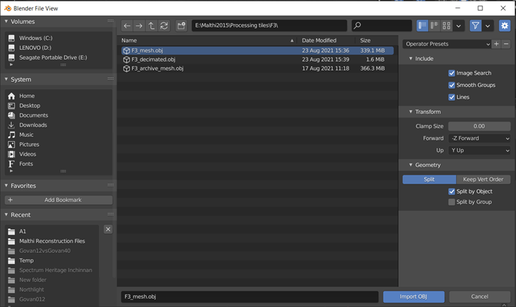
Note: Notice on the file import screen that, under ‘Transform’, there are a few dropdown menus. You’ll notice that it is automatically set to ‘-Z Forward’ and ‘Y Up’. This is typical of many 3D modelling software packages, like Maya. However, think back to how our dataset appeared when imported into CloudCompare or MeshLab – the Malthi dataset would appear as if from a bird’s eye view above the site. In CloudCompare, we would often use the ‘Z values’ of our point cloud to visualise the dataset so that we could identify features based on their height. Most of the software we’ve used so far uses the ’Z up’ principle. It’s not entirely clear how this difference came about, except perhaps that, if we think of drawing in two dimensions, or a mathematical plot in two dimensions, X is often the Left-Right axis and Y is the Up-Down axis. In moving from this 2D point of view, the addition of a third dimension would become essentially ‘Depth’, as the Z axis has in these 3D modelling software packages. If we think of a geospatial dataset or map, it makes more sense for the X and Y axes to be represented by North/South and East/West axes, with the Z axis representing the height above sea level. It is important to be aware of these differences, because as you import our Malthi dataset into Blender with these preset import options, your mesh will initially appear to be sideways in the 3D space. If your preference is for Z up, you can change the ‘Up’ setting to Z before importing your meshes, but be aware that you will need to change this for every subsequent import. Because we will be exporting another file containing the UV-unwrapped low-resolution mesh associated with the newly created normal maps, you may wish to leave it at its default setting for now and wait until Exercise 4 to re-align the data to the Z-up position. In the examples below, the data has been left in the default ‘Y-up’ position.

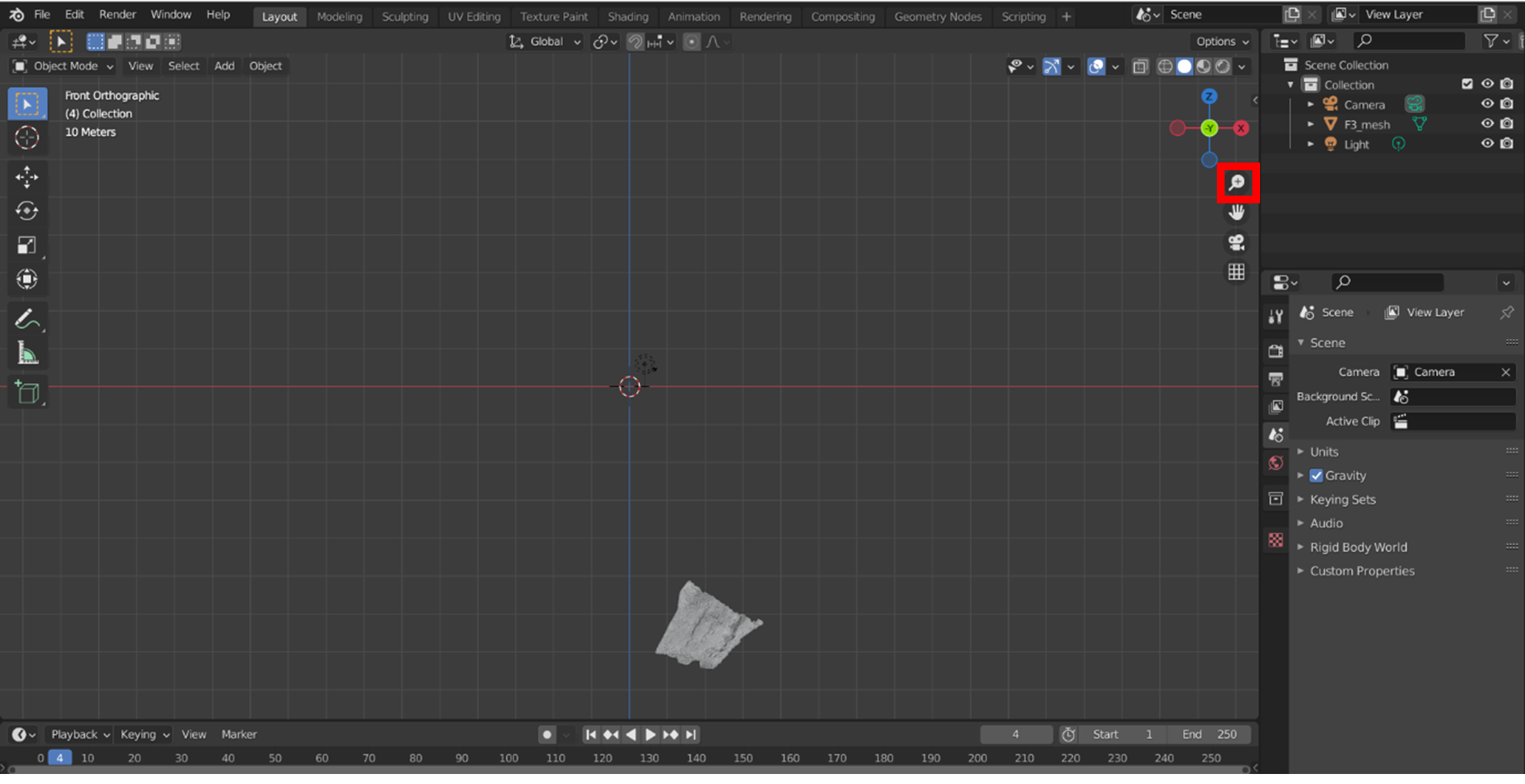
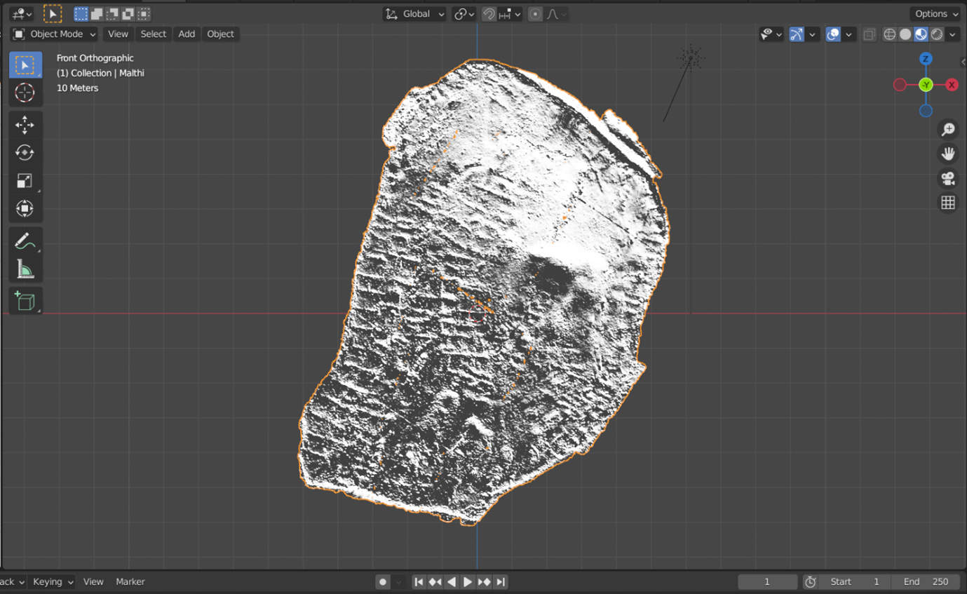
Now import your first original resolution mesh and its associated decimated mesh. At this point, you may need to zoom out to find your mesh, because it is still georeferenced in relation to the other segments of the original Malthi dataset (though it is not reflecting the Global coordinates as it originally when imported into CloudCompare, it is reflecting the ‘Global shift’ of coordinates you performed to move the dataset into a local coordinate system). As you can see in the image below, the segment of data shown is the south-east corner of the site of Malthi, so it is a substantial distance away from the ‘Origin’ at the centre of the screen (the red and white circle). You can zoom out by either using your mouse-wheel or by left-clicking and dragging the magnifying glass in the top right area of the viewport (highlighted by a red box).

Notice that by default, you are in ‘Object Mode’. This means that any changes you make will be on an object-based level, rather than a face or vertex-level change. You should avoid moving or rotating the meshes themselves while in this mode, as this will alter the georeferenced position of the mesh. Panning or rotating the view of the mesh, however, will not affect its georeferenced position. If you want to put all of the pieces of the decimated Malthi dataset together easily once they are normal mapped, it is best to keep the georeferenced mesh in this position.

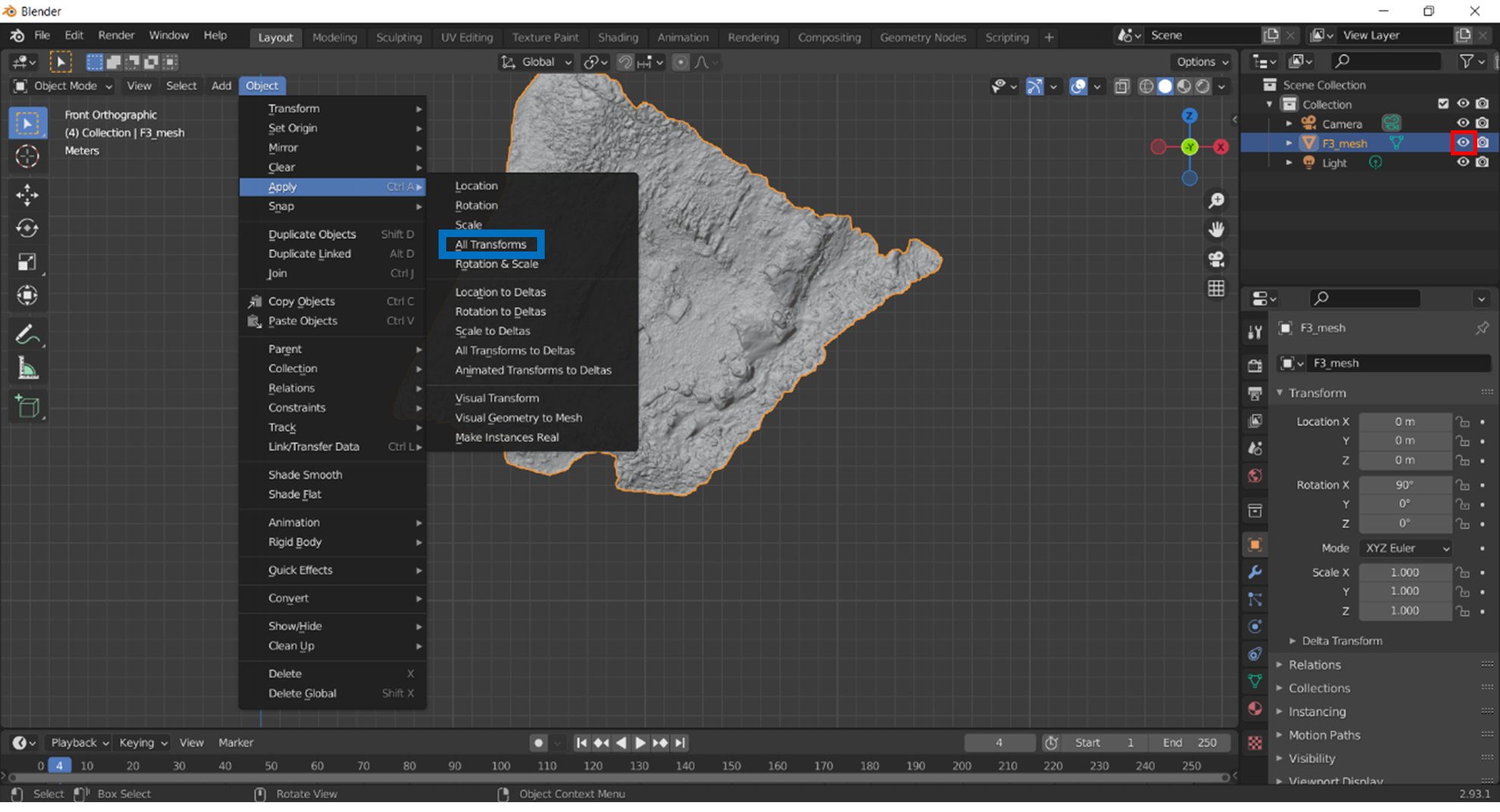
As you import each mesh, ensure that the current mesh is highlighted in the ‘Scene Collection’ window, then navigate to the ‘Object’ menu in the top left corner, select Apply, and All Transforms (highlighted with a blue box below). Because we are working with reality captured data, this will ‘set’ or ‘fix’ the data in place. This is essential for the normal mapping to work in later stages. You can now ‘turn off’ the original resolution dataset by clicking the ‘eye’ symbol next to the name of your high resolution mesh (surrounded with a red box below). To orient your mesh to the bird’s eye view that we are accustomed to, use the 3D axis above the ‘Zoom’ tool to orient it. If you imported the mesh as ‘Y-up’, click on the green ‘Y’; if it aligns to ‘-Y’, click it again and it will flip. If you imported the mesh as ‘Z-up’, click on the blue ‘Z’.

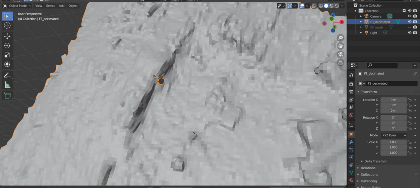
At this point, it is worth examining your decimated mesh, as you may have noticed some small holes when it was generated by Instant Meshes. Blender has some navigation short cuts that can be difficult to get used to. To pan your view, hold down ‘Shift’ and click and drag your middle mouse button. Holding and dragging your middle mouse button will rotate your view of the mesh. If you click on your decimated mesh while in object mode, orange lines should outline the boundaries of the mesh and highlight any holes that are less visible.

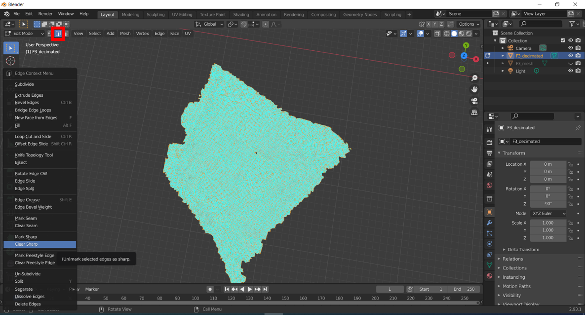
There are a couple of methods that will allow you to fill these holes. First, switch from ‘Object Mode’ to ‘Edit Mode’. You will notice that the edges of your quads will become highlighted, as you can see below. This is a by-product of the creation of the mesh in Instant Meshes. Ensure that ‘Edge Select’ (highlighted in the red box below) is on. With the decimated mesh selected (you can also press ‘A’ to highlight what’s visible), right click anywhere in the viewport and select ‘Clear Sharp’.

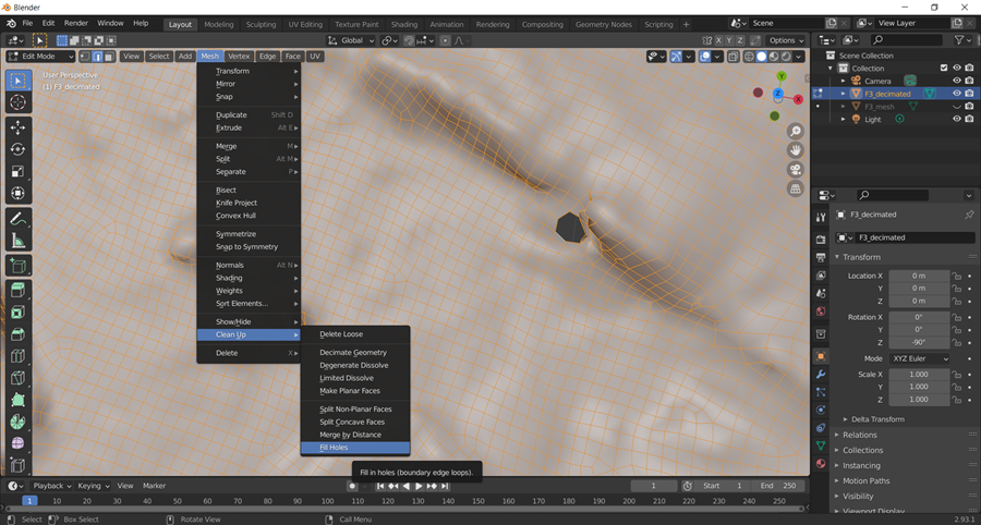
To fill the hole visible towards the centre of this mesh, you can try using the automatic ‘hole fill’ algorithm by selecting the mesh (by hitting ‘A’, for all), and navigating to ‘Mesh > Clean Up > Fill holes’. This will not always work, if the hole is large or complex in shape.

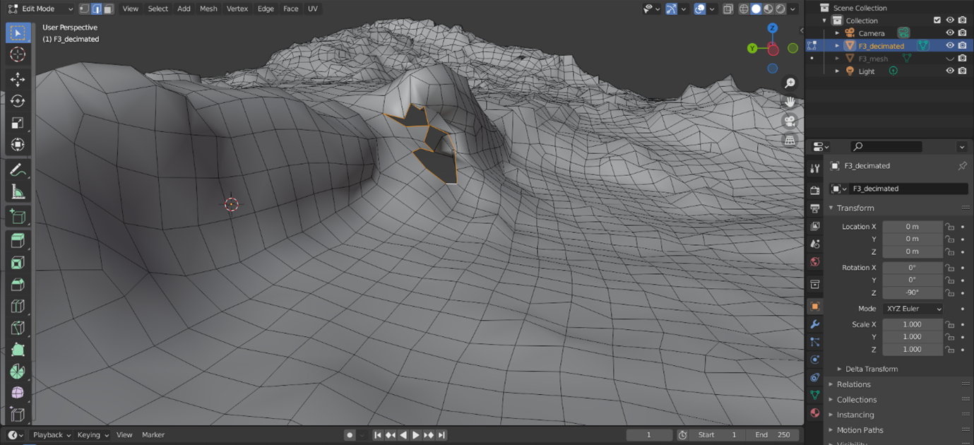
To manually fill the hole, ‘Alt + Left Click’ in the hole. This will select the edges of the hole. Then, press ‘Alt + F’. The software should automatically fill the hole with triangles. Once all holes are filled, switch back from Edit mode to ‘Object Mode’.

Try it yourself! Which of these options worked best to fill any holes in your decimated mesh? If something didn’t work, why do you think caused it?

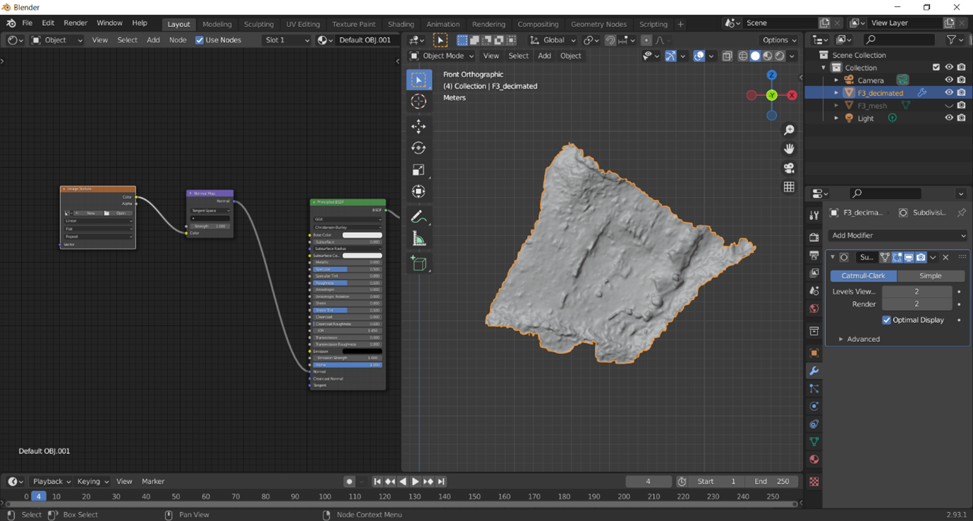
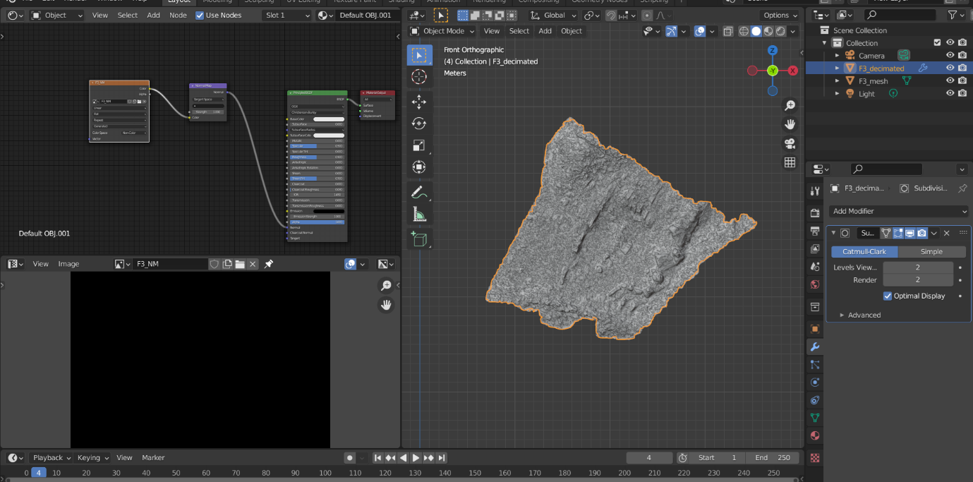
Now we need to smooth our Decimated Mesh so that the mapping of your high-resolution normals onto the low-resolution geometry transitions more smoothly between mesh faces (for further insight into this process, see this blog by Carlos Lemos). Once in Object Mode, right click anywhere in the viewport and select ‘Shade Smooth’. To further smooth your decimated mesh, Next, you may want to add a modifier called ‘Subdivision Surface’. Access this by selecting the ‘wrench’ icon in the ‘Properties’ area of the Blender interface (highlighted with a red box below). Set the ‘Levels View’ to 2.

Now we need to start to build the image file that we will be projecting the normal map onto. Move your mouse to the top left of the screen, just under the Blender symbol on the toolbar, and your mouse should change to look like crosshairs. Click this and drag your mouse to the right to split your screen. In your new window, open the ‘Editor Type’ menu (highlighted in a red box below) and select ‘Shader Editor’. This is where we will be adding nodes.

Nodes are a form of programming; in Blender, they are primarily used for shaders and materials, though they can also be applied to lighting and animation. Each node you add will be specialised to perform a specific function. These nodes can be combined in different ways by making connections between them. For creating a Normal Map, we only need to add two nodes – Image Texture and Normal map. When you first enter the Shader Editor, there should be two nodes already there – Principled BSDF and Material output. To remove the additional ‘Node’ menu on the right side of the Shader Editor, click in the Shader Editor viewport and then press the ‘N’ key. To add the ‘Image Texture’ node, press ‘Shift and the A key’, press the ‘S’ key for Search, type in ‘Image’ and hit Enter when ‘Image Texture’ is highlighted in blue. Use your mouse to move and place the node by left-clicking.

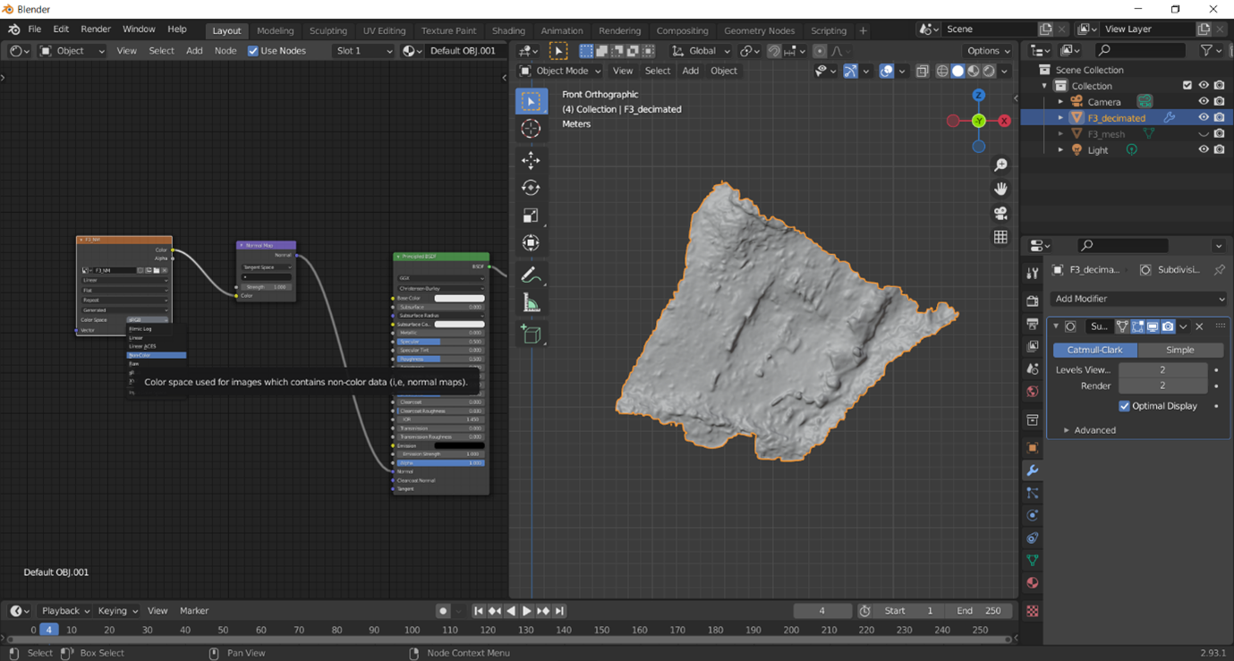
Repeat these steps, except this time search for ‘Normal Map’ (not Normal). Place the node between Image Texture and the Principled BSDF nodes. If we look at the ‘Image Texture’ node, we will see that there are two traits on the right side of the box – Color and Alpha. Click and drag the small circle next to ‘Color’ and drag this to the circle next to ‘Color’ on the left side of the ‘Normal Map’ node. Next, connect the ‘Normal’ option on the right side of the ‘Normal Map’ node and connect it to the ‘Normal’ option on the Principled BSDF. Your nodes should be connected as they are in the image below.

Now, let’s create our image file. On the ‘Image Texture’ node, left-click ‘new’. This will prompt you to name and set the size of your normal map. Ensure that you follow the naming convention you set out at the start of this Exercise. You can create a 4K texture if you set the width and height to 4096 px. Click OK. There will now be new options available on your ‘Image Texture’ node, and it will be renamed to match your image name. Change the ‘Color Space’ drop down menu to ‘Non-colour’.

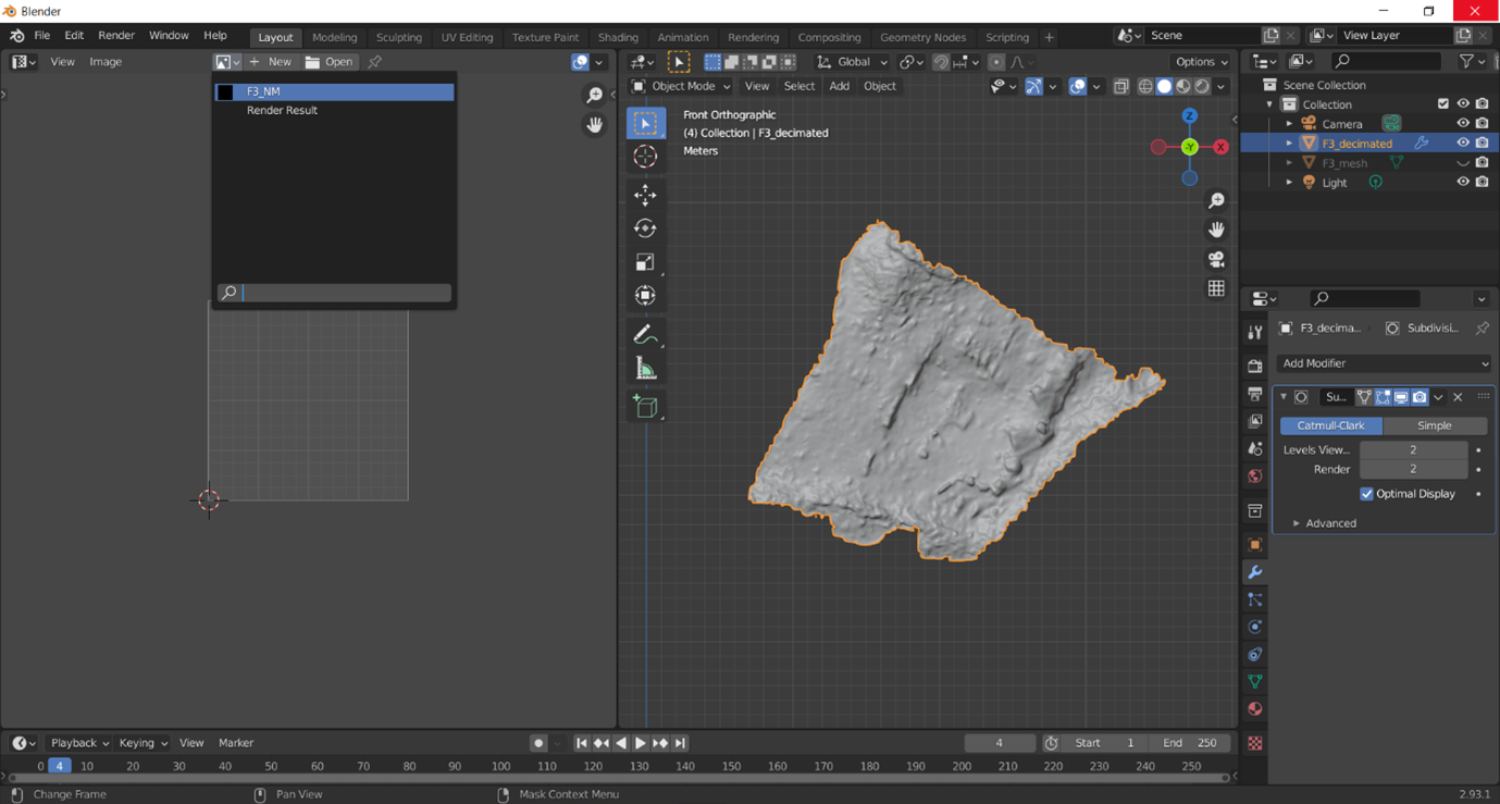
Now we need to UV Unwrap our decimated mesh. UV Unwrapping comprises of unfolding and flattening your 3D mesh into a 2D image. While similar in concept, it is a bit different from unwrapping a gift, because you cannot have any overlap or folds in your 2D ‘paper’. To get started, change your ‘Shader Editor’ window to ‘UV Editor’ and set the image as the one you created in the Shader Editor. This is where your ‘unwrapped shapes’ will appear.

In your ‘Layout workspace’ viewport with your decimated mesh, change to ‘Edit mode’. Now there are a few ways to unwrap your UVs – you can either create your own seams, from which you want the software to unwrap your UVs, but it takes practice to identify the best way to ‘cut’ these, especially in a mesh with such complicated topography, even when decimated.

Note: If you want to create your own seams, ensure that your Layout workspace is in Edit mode with ‘Edge select’ enabled. Left click to select individual edges; you can also ‘Ctrl + left-click’ anywhere on the mesh and it will find the shortest path between your starting and ending points. When you are happy with your seam, right click anywhere in the layout space and click ‘create seams’. Once you are happy with your seams, change to ‘Face Select’, press the ‘A’ key to select all, the ‘U’ key to unwrap.

To use the ‘Smart UV Project’, put your Layout workspace into ‘Edit mode’ with the decimated model visible, change to ‘Face Select’, press the ‘A’ key to select all, and then Navigate to ‘UV > Smart UV Project’. Accept the default options and press ‘OK’. Your unwrapped mesh should appear in your UV Editor viewport.

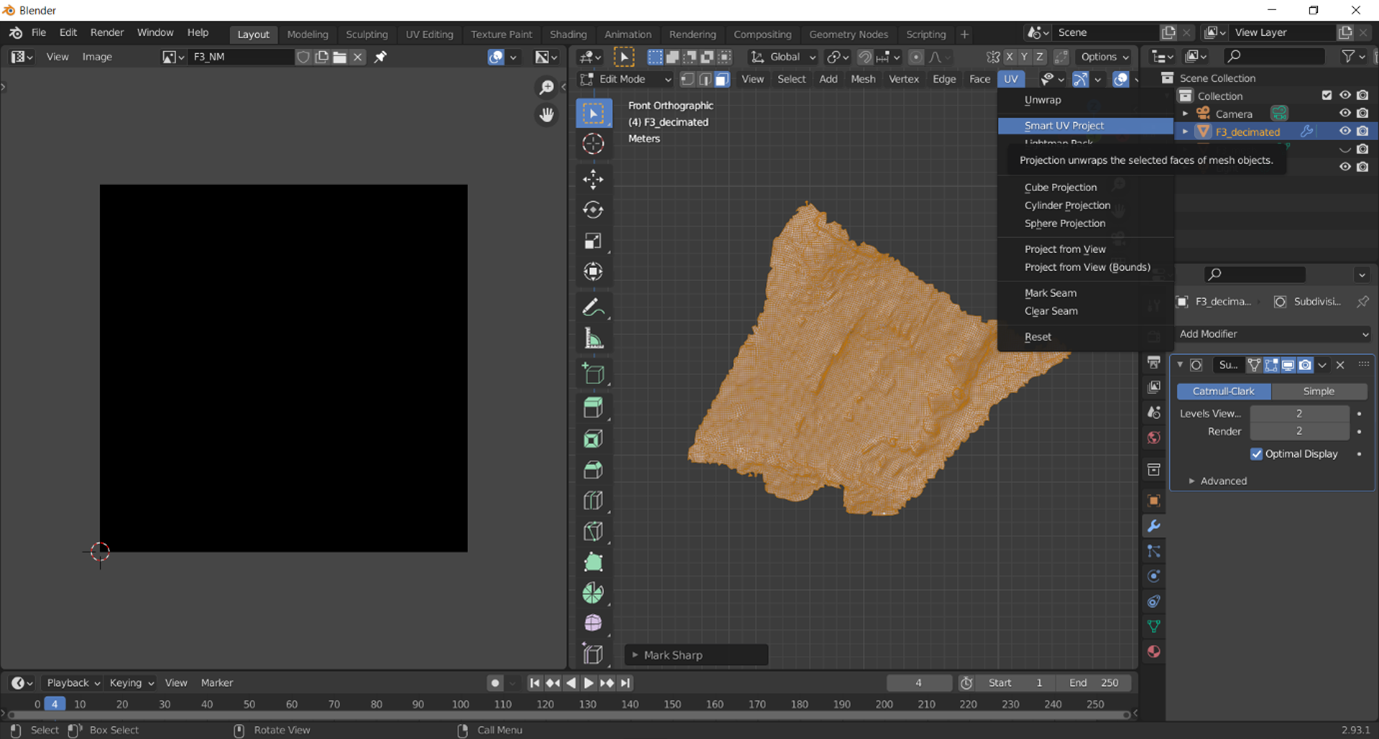
While the UV map generated by the ‘Smart UV Project’ tool will not be pretty, necessarily, and will create many islands, these still result in very good normal maps. Use the ‘UV Selection Mode’ from the UV Editor toolbar if you want to select, move or rotate any individual UV.

Think and Respond: Watch part of J Middleton’s tutorial video (at least from 25:45 – 32:48). Did you create your own seams? How did they turn out? (and if they didn’t, why do you think J Middleton’s seams worked for the UV map?) If you used the Smart UV project, can you see why this would be disadvantageous for other projects (especially those incorporating colour)?

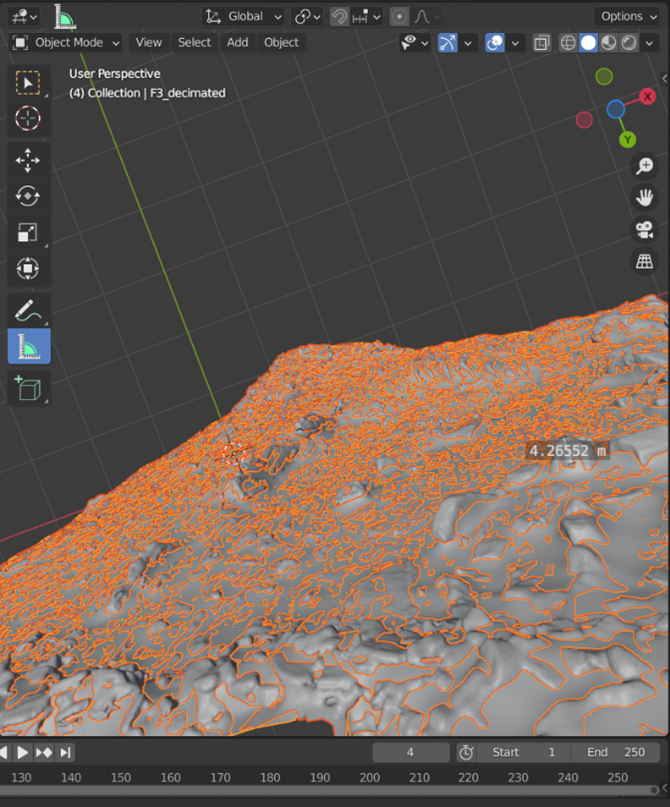
Now, put your Layout workspace into ‘Object Mode’ if it isn’t already, and make your high-resolution model visible again. Use the ‘Measure’ tool from the toolbar of green icons to identify the distance between your decimated mesh and your original mesh by enabling the tool, left-clicking a place on the mesh where the decimated mesh is visible through the high resolution mesh, and drag your mouse to the point on your high-resolution mesh that appears to correlate to that decimated feature. Take note of this, as this will help find the best ‘extrusion’ level to set in the baking settings (see Jayanam’s tutorial here).

Split your UV editor window into two by hovering your mouse over the top left corner of the window until the crosshairs appear. Then click and drag to create a new subdivision of the window. Change one of these UV Editor windows to ‘Shader Editor’. First, highlight your high-resolution mesh in the ‘Scene Collection’ area and ensure that all nodes in the Shader Editor are unhighlighted by left-clicking anywhere in the Shader Editor. Now highlight the decimated mesh in ‘Scene Collection’ and ensure that the ‘Image Texture’ node is highlighted by left-clicking it. Be sure that this is the only node that is highlighted.

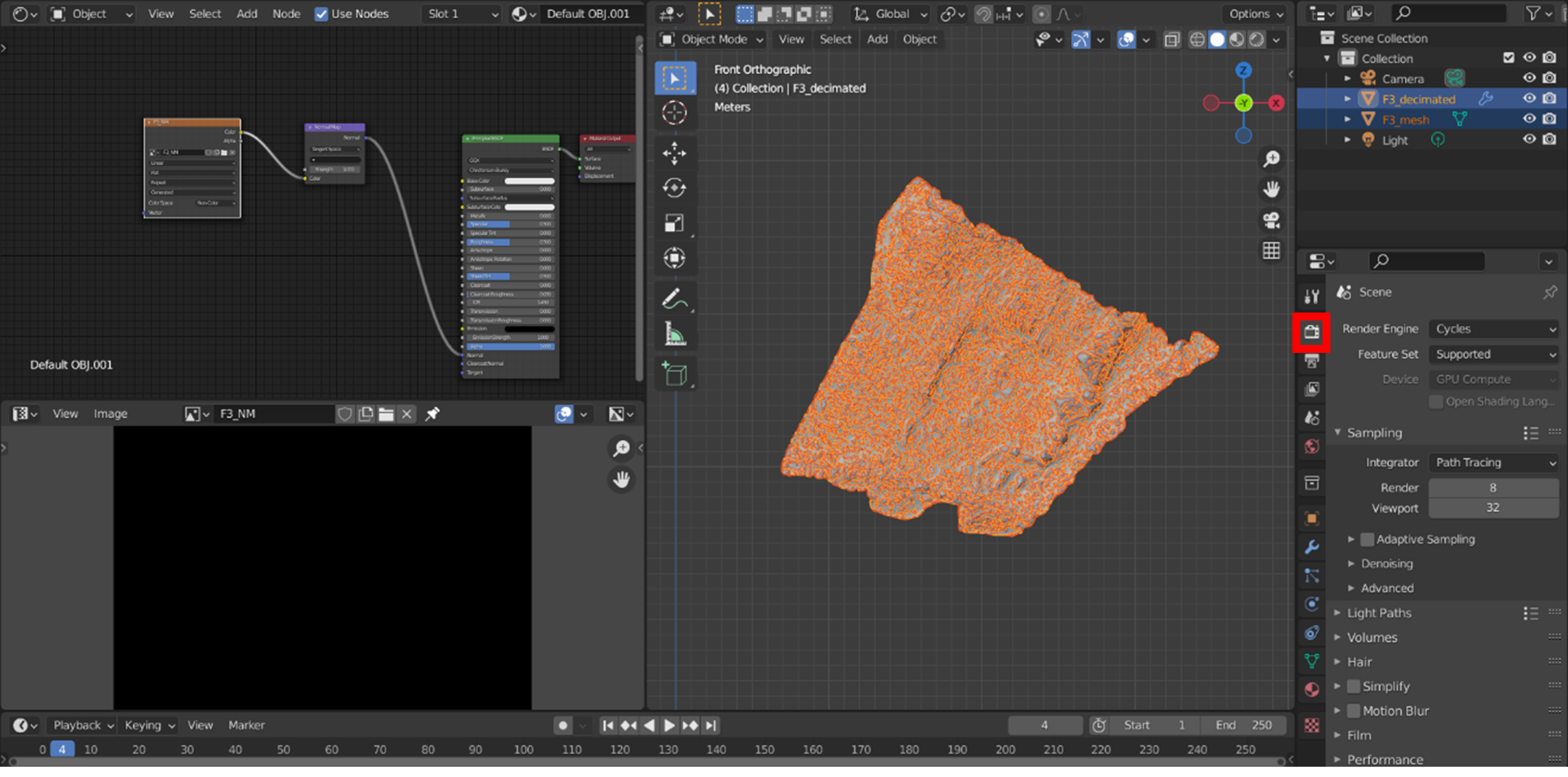
For the next steps, the order in which you click certain features is very important or the bake will not work. In Scene Collection, first, left-click on high resolution model first to highlight it; then Ctrl + left click the low poly model in Scene Collection so that both meshes are highlighted. The original mesh should be a darker orange colour while the decimated mesh should be a lighter orange. In Properties, you should select the ‘Render Properties’ tab (surrounded with a red box below) and change the Render Engine to Cycles. You can set your ‘Device’ to GPU compute if you have specialised graphics card, but it is not necessary.

There are a number of settings that can be changed in these properties. If you leave most of these at their presets, it will take a significant amount of time to process the Normal map. For those with impressive computers, you could probably run each dataset with these settings. If you want to test how long it will take, save your Blender file before running the Bake in case Blender crashes.

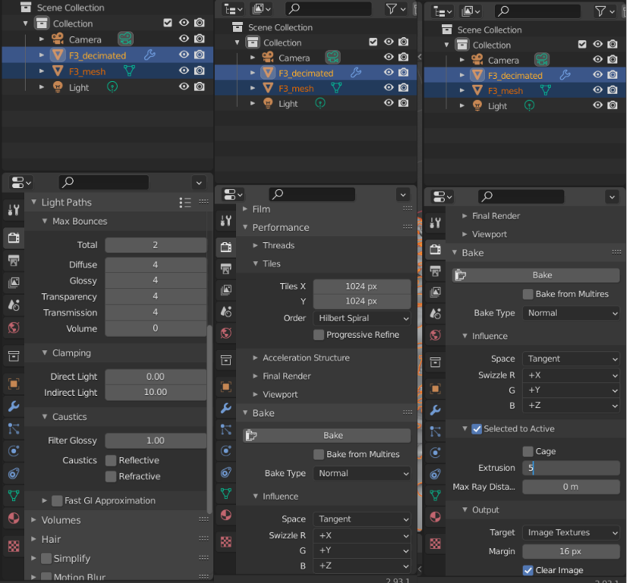
For the rest of us, J Middleton’s YouTube normal baking tutorial recommends the following settings: Under ‘Sampling’, you can set ‘Render’ to 8. Under ‘Light Paths; Max Bounces’, the total can be set to 2, while Diffuse, Glossy, Transparency, and Transmission can be set to 4. Under Caustics, can unselect Reflective and Refractive. Under performance, set the ‘Tiles X and Y’ to reflect the px size you set your Normal Map image to originally (4096 px if you created a 4K image). Under Bake, set ‘Bake Type’ to Normal, ensure that ‘Selected to Active’ is checked, and that, under Selected to active, set the ‘Extrusion’ to reflect the height distance between the original mesh and the decimated mesh. While online tutorials will often recommend somewhere between 0.1 and 0.5, our measurements earlier have indicated that we should set this to 5m to achieve the best results (see Jayanam’s tutorial for further information). Press the ‘Bake’ button when you are satisfied with the settings (if you would like further information on the different settings, see Blender’s Documentation regarding the Cycles Rendering engine here).

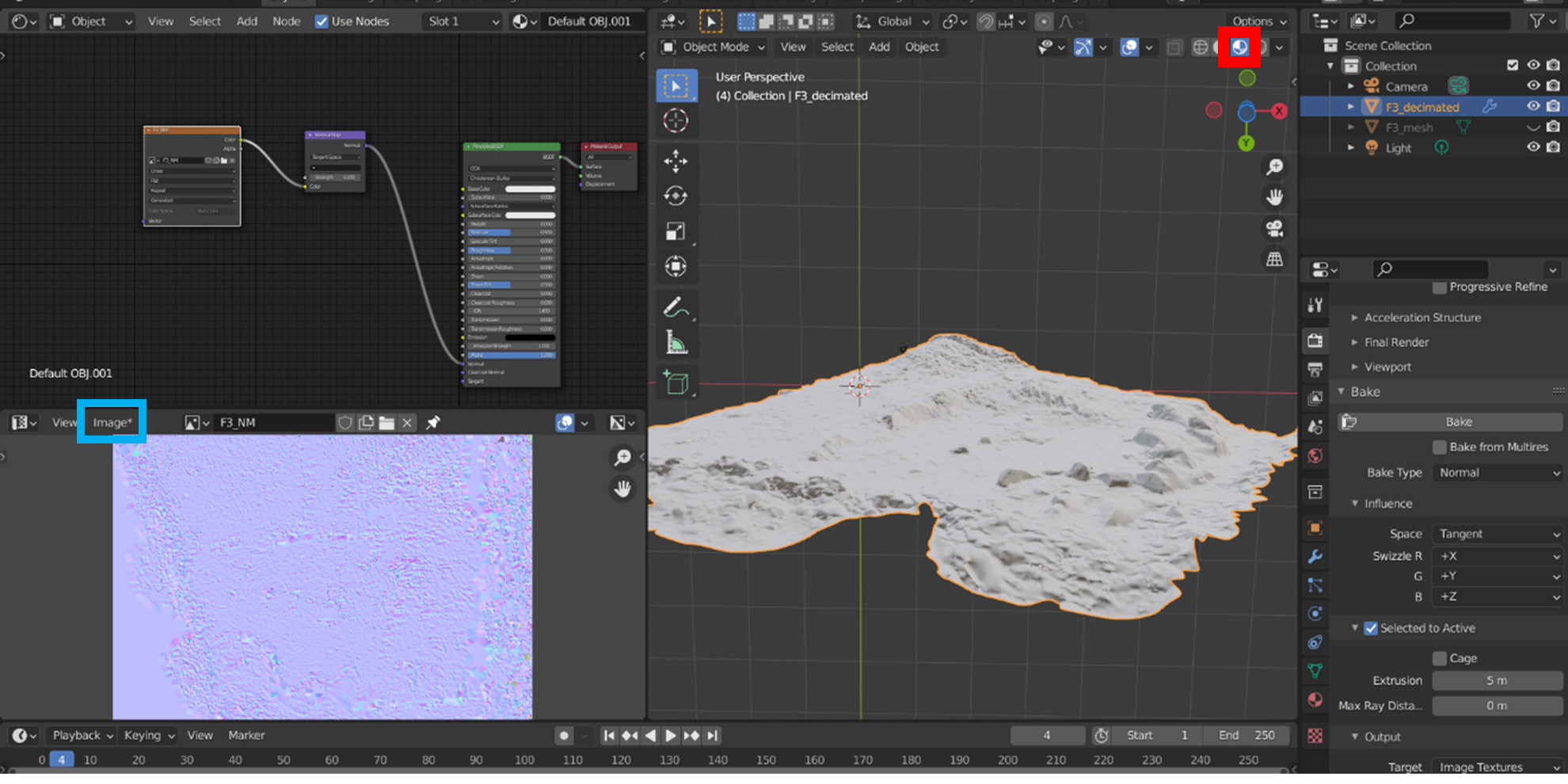
After it has finished processing, hit ‘Viewport shading’ in the Layout workspace to see if it has mapped the normal map correctly.

Try it yourself! Try changing the Viewport shading options in your 3D Viewport – you can find this in the dropdown menu just to the right of the ‘Viewport shading’ button highlighted in the image above. How does this change the appearance of your decimated mesh and the normals?

Once you are happy with your mesh and the normal map, you can save the normal map. In the ‘UV Editor’ toolbar, click ‘Image*’ (highlighted with a blue box in the image above) and then ‘Save As’. Save the image in the same folder in which you intend to save the decimated model. Remember that, if you move the normal map after the decimated model has been generated, they may become disassociated.

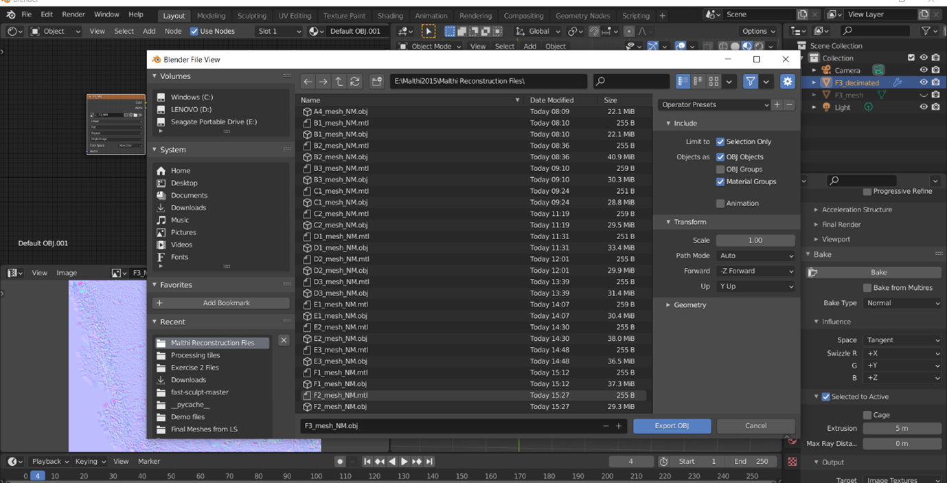
Now export the decimated model. Ensure that only the decimated model is highlighted in the ‘Scene Collection’. Then, navigate to ‘File > Export > OBJ’. A dialog box like the one pictured below will appear. It is important to note the options available on the right hand side. Ensure that ‘Selection only’ is checked, and that both ‘OBJ Objects’ and ‘Material Groups’ are checked. This will ensure that the Normal map is automatically connected to the correct OBJ file in later steps.

Think and Respond: Examine your decimated mesh with the normal map applied and compare this to the original mesh by turning their respective layers on and off. Do you see the benefit in creating the normal map? Do you think this will be easier to model on than the decimated mesh alone? Why?

n.b. In a real project, you would now go back and deploy this routine over all the other meshes you want to incorporate into the reconstruction. You would create a new Blender file and import each mesh, highlight them all in the ‘Scene collection’ box. In Object mode, by navigating to ‘Object > Join’, you would join all of these meshes together in a single mesh, which could then be exported separately. See an example of the results below.

Exercise 3 Resources:

Blender. “Common Shortcuts.” Blender 2.93 Reference Manual. Last updated 25 Aug 2021. https://docs.blender.org/manual/en/latest/interface/keymap/introduction.html#common-shortcuts.

Jayanam. 2020. “Blender Bake Normal Map Beginner Tutorial.” YouTube. Uploaded by Jayanam, 10 December 2020, https://youtu.be/DQPjIGncXcM.

KatsBits. 2015. “Bake Normal Maps With Cycles.” Website. 9 May 2015, https://www.katsbits.com/tutorials/blender/cycles-bake-normal-maps.php.

Lemos, C. 2020. “Tutorial: How Normal Maps Work & Baking Process”. 80.LV Article. 24 March 2020. https://80.lv/articles/tutorial-how-normal-maps-work-baking-process/.

Middleton, J. 2020. “Photogrammetry Meshroom Clean up Mesh in Blender High-Poly to Low-Poly Normal Map Baking.” YouTube. Uploaded by J Middleton, 21 October 2020, https://youtu.be/MrUVeV0wsH8.

Mister P. MeshLab Tutorials. 2011. “Cleaning: Basic Filters.” Youtube. Uploaded by Mister P. MeshLab Tutorials, 25 May 2011, https://youtu.be/aoDLrXp1sfY.

Back to Exercise 3 Part A

Continue To Exercise 4