Exercise 1

Part C: Prepare your data – extracting what you need

Step-by-step instructions for this part of the exercise can be found here.

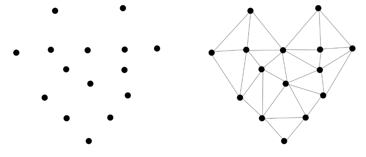
For the purposes of our exercise, we are primarily interested in the foundations of the buildings at a minimum, as we wish to understand what it would be like to navigate the built space. We also decided that we want to work with meshes rather than point clouds because, while point clouds are aesthetically pleasing and technically the most accurate part of a 3D dataset, point clouds are not the traditional basic unit of construction used in 3D modelling; instead, we will be working with meshes. Like the SfM photogrammetry models you viewed in the previous step, a mesh is formed when triangular polygons are generated between the points of a point cloud until a ‘solid’ mesh is created. The point cloud becomes the vertices of the mesh. This means that, to progress further, we need to translate from a point cloud to a mesh. Conceptually, this means we need to get our point cloud to only include points we want forming the meshed surface. Meshing is the software essentially playing connect-the-dots to draw a picture. If you include dots (laser scan points) that you don’t want to have be part of the picture the software is drawing, it will include them anyway and your picture will look pretty strange.

On the left, a series of 'points' - on the right, the dots have been connected to form a meaningful 'mesh'.

For most projects, you won’t need or want everything in the point cloud, as we noted above. Begin to prepare your data by getting rid of things you don’t need and keeping those that you do need. When working with large datasets, we recommend running through these preparation steps with a small sample area the first time through to make sure the results are satisfactory. Once you’re happy with the process, you would go back and run it on the whole dataset. We’ll follow this ‘test, assess, deploy’ strategy throughout this exercise.

Step 1: Segment your test region

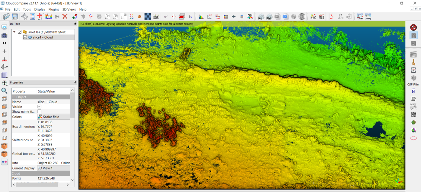
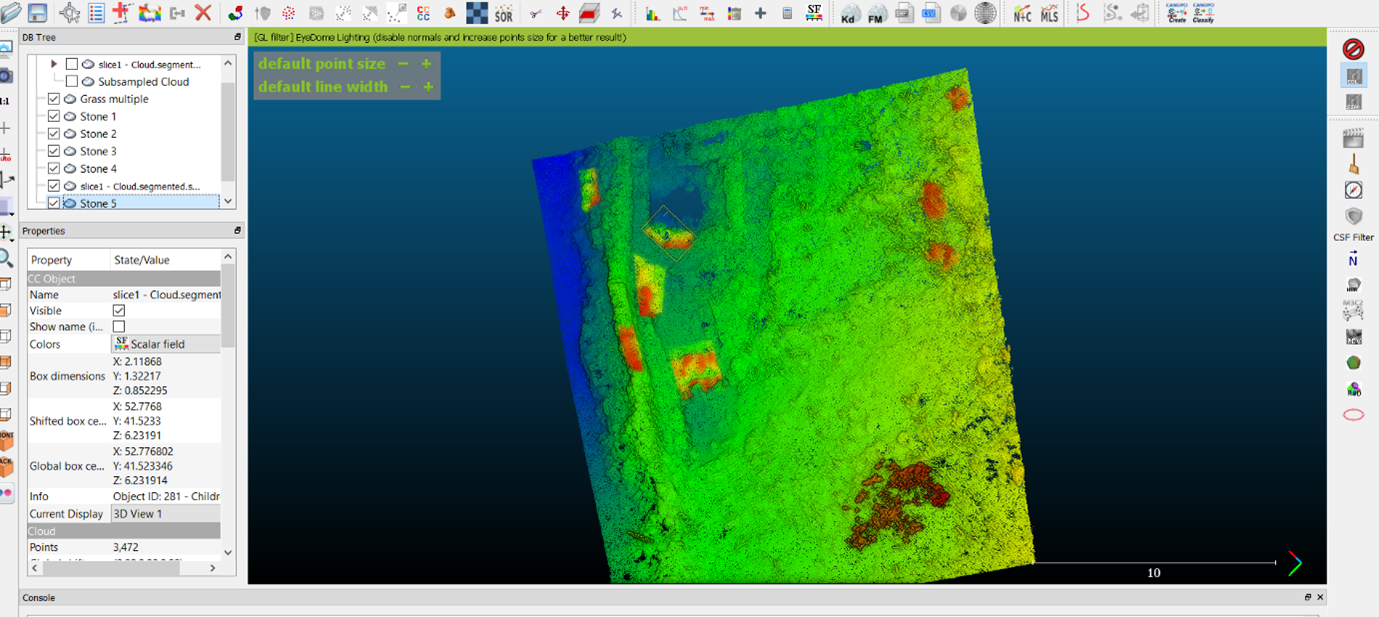
First, open Profile Slice 1, apply the EDL shader and create a Scalar field based on the Z coordinates as you did above. Look for an area that contains some data you will need and some data you won’t need. If we look at the middle region of Profile Slice 1, we can see that there are areas with grass, trees, the boundary wall, and the foundations of buildings. Keep this area small so that things run quickly and you can test rapidly.

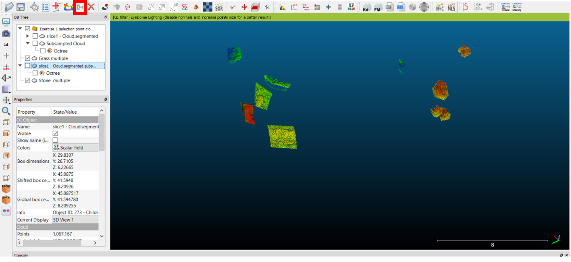
A screenshot of slice 1 of the Malthi dataset visualised with EDL shader and height values as a scalar field. This will be the target area for sampling, as it has grass, trees, and structures in a small area.

To section this area away from the rest of the data, we will be using CloudCompare’s ‘Segment’ tool. First, ensure that the ‘slice1 – Cloud’ layer is highlighted in the DB Tree. Find and click the ‘Segment’ tool on the toolbar (or under the ‘Edit’ drop-down menu) – it looks like a pair of scissors.
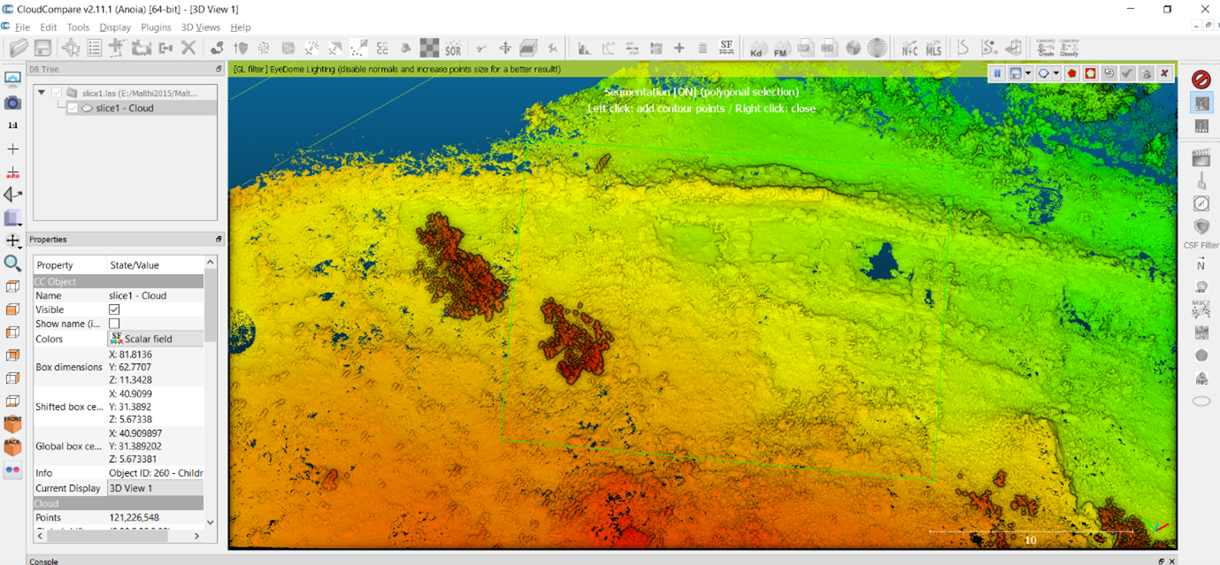
A small toolbar will appear in the top right corner of the toolbar, and basic instructions will appear in the top centre of the screen.
Left-click to begin drawing a boundary around the region you want to work with – as you continue to add points, a green-lined polygon will expand to show the bounds of the region you have selected. Once you are happy with the region you have selected, right click anywhere in the viewer to finish the polygon.

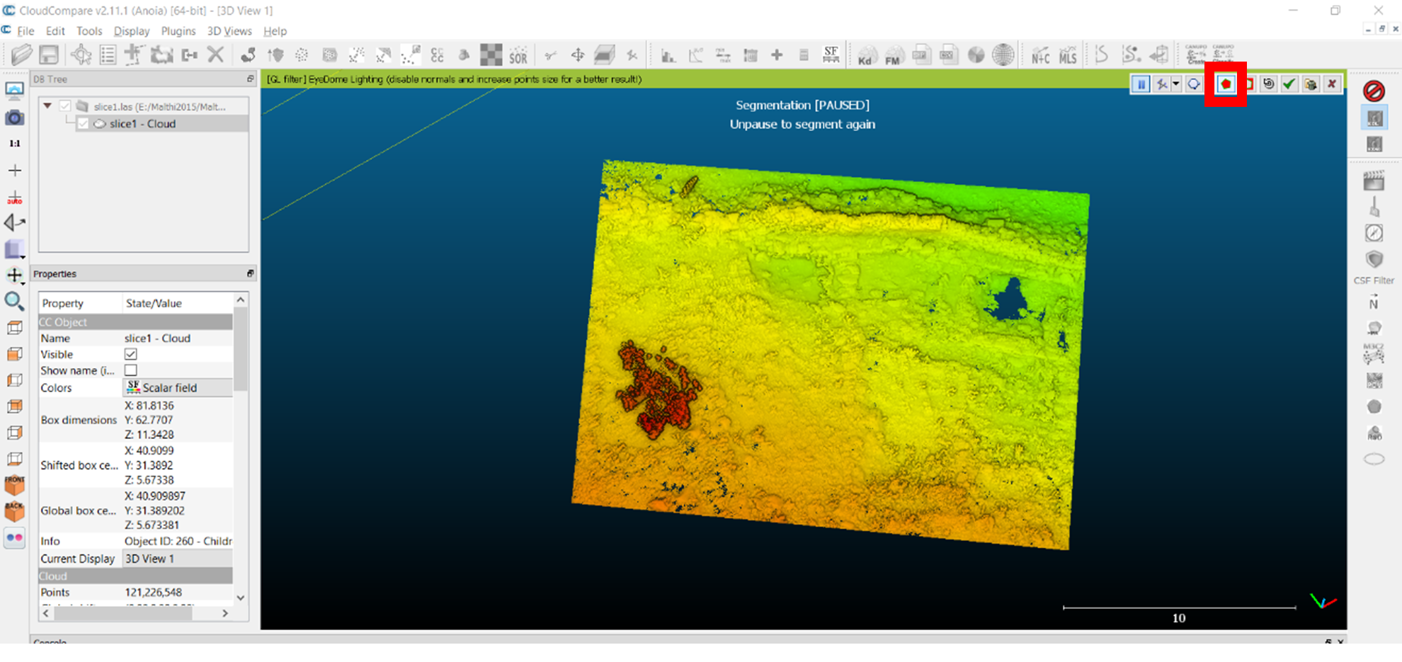
A screenshot of the Slice 1 of the Malthi dataset. A faint green box generated by the segment tool is visible around the data in the middle of the screen.

Because we want to keep the area inside our polygon, select the ‘Segment in’ button from the small toolbar (highlighted with a red box below). This will provide you with a preview of the selection you’ve made.

Selecting 'Segment in' (the button surrounded by a large red square in this image), a preview of your selected test dataset is generated. Clicking the green tick button (three buttons to the left of the 'Segment in' button) will approve this division and put the rest of the data on a different layer.

Once you are happy with your selected test dataset, click the green tick button (three buttons to the left of the ‘Segment in’ button) to approve. The software will then put the rest of the data on a different layer, ‘slice1-Cloud.remaining’ – you can delete this from the DB Tree to save memory, simply uncheck the box next to it so that it is no longer visible, or save the remaining data as a separate BIN file to work with later. Save your current dataset as a BIN file by clicking on its layer in the DB Tree and navigating to ‘File > Save’.

Step 2: Set your Level of Detail

What spatial resolution is needed for your project? What is manageable? This may be a compromise! Reduce the resolution to the level of detail you need. Keep in mind that the total number of points in the Malthi dataset exceeds 650 million points, Profile Slice 1 contains over 121 million points, and the segment generated in the image above contains about 39 million points. The CloudCompare meshing algorithm will generate twice as many mesh faces, and, often, meshes of 10 million faces are difficult to handle on mid-range computers. This segment is still quite a substantial dataset! Our next option to thin out the point cloud is to subsample it. This will decrease the number of points in your point cloud based on different algorithms that are available.

First, navigate to ‘Edit > Subsample’. There are three sampling methods you can try:
- Octree – this is essentially a type of stratified sampling. The algorithm breaks up the point cloud into eight ‘boxes’ based on the bounding box (the yellow 3D box surrounding your sample), then breaks those eight boxes into eight more boxes (etc), and subsamples the clouds in each octree; however, this is still somewhat unpredictable in terms of how points are selected in those randomised boxes. - In the dialog box, you have the option of choosing how many times the boxes will be ‘broken up’ – the closer the sliding scale is to ‘max’, more boxes are generated, and fewer points are lost from each.
- Random sampling – truly random sampling – so you may lose more detail in some areas than others. - In the dialog box, you can use the sliding scale to choose how many points are left.
- Space method – this samples based on the ‘distance between points,’ so is particularly useful if you have specific accuracy needs. The dataset is scaled in metres.
  
  Hint
``` As noted in the metadata report, 0.025 spacing between points still allows for individual stones to be seen, though we will lose substantial detail upon creating the mesh. ```

Try it yourself! Try each of the subsampling methods on your test point cloud. Be sure to duplicate your point cloud a few times before doing this; simply highlight your sample and navigate to ‘Edit > Clone’. Rename the layers according to the sub-sampling method to be particularly organised, by double clicking the name of the layer in the DB Tree and giving each an informative name. Write a short paragraph describing what differences you noticed between the different methods and which you think is best for this project.

Step 3: Prepare your data – remove noise and unwanted data points

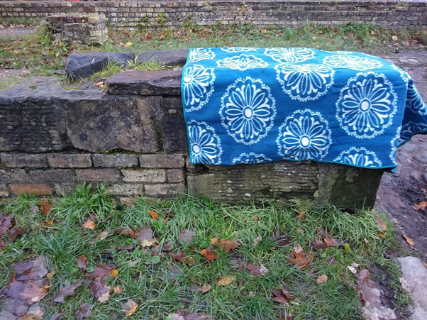
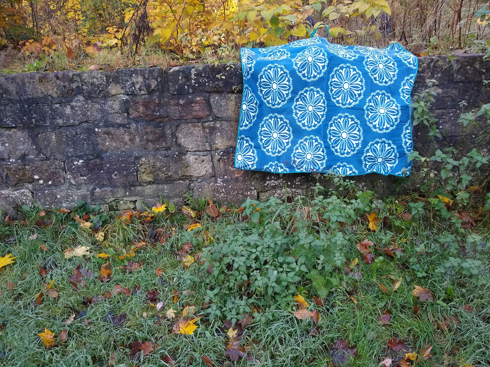
The next step is to clean your point cloud to remove the data that represents objects / items you don’t want in your reconstruction. There is likely a great deal of data included that you do not want incorporated into the mesh – in this case, the patches of grass and the trees growing on the site have been preserved in the dataset. Refer back to what we said about meshes and connecting the dots. To visualise creating a mesh, imagine that you have a blanket and that there is a wall in front of you, clear of any vegetation on either side of the wall. In this case, it would be easy to drape the blanket over the wall and still identify the shape of the wall. If, on the other hand, there is grass and moss growing on top of the wall, a tree growing close to the wall, and tall grass on either side, draping your blanket across the wall may result in a lumpy ‘mesh’ and make it difficult to identify the detail of the wall.

A wall clear of most vegetation is easy to cover with a blanket, simulating the accurate creation of a 3D mesh of the wall.

A wall with significantly more vegetation surrounding it, which does not allow the blanket to lie flat, indicating that this would affect the 3D mesh of such a structure.

Think and Respond: Why is it essential to remove the vegetation from the point cloud, in this case?

Now let’s think about the character of what you are trying to remove. How different is the shape of a tuft of grass compared to a smooth stone wall? How does their difference in shape affect the organisation of the points comprising these features in the point cloud – how are the points situated in relation to one another for each feature? If the point cloud for a tuft of grass is organised quite differently from the point cloud of a stone wall, you may be able to ‘teach’ the software to automatically tell the difference between these sets of points. If they are quite similar you will have to take a more manual approach (see Brodu and Lague 2012 and CloudCompare documentation on the CANUPO plugin).

Think and Respond: Can you think of other features that you may want to separate in other hypothetical laser scan datasets? Are they quite similar to each other in terms of shape, or quite different? How would you describe these similarities/differences? What would the benefits be in separating these features?

Lucky for us, vegetation and walls usually look fairly different in laser scanned data, so we can attempt some automated cleaning.

There are a few automated tools to remove these unwanted features in CloudCompare.

CANUPO: This is a plugin that allows you to create classifiers based on your dataset to classify different types of features based on their shape.
- To begin, you first need to clone your point cloud to have an intact backup.
- Next, use the ‘Segment’ tool to isolate the different features you want to distinguish between. Left click around the feature you wish to isolate; right click to finish the shape. Click the ‘segment inward’ button. Make sure that these sampled areas are as ‘clean’ as you can manage. If you are trying to separate grass from stone walls, ensure that the point cloud sample you take only has grass or stone wall in it. If you are happy with what has been selected, click the checkmark in the Segment toolbar and the segment will be allocated to a new layer in the DB Tree.
- Because this process is essentially creating a Machine Learning dataset, you may need to segment out multiple well-defined, but varied in appearance and size, examples of ‘grass’ and ‘stone’ so that the AI can better identify the many different forms grass and stone can take. Rename the layers you create with a descriptive name. Once you have a number of ‘grass’ samples, highlight each of these layers in the DB tree, and navigate to ‘Edit>Merge Multiple Clouds’. Repeat this with the ‘stone’ samples so that, in addition to your primary point cloud, you have two clouds: one containing your examples of stone walls or stone, and one containing your grass/vegetation samples.

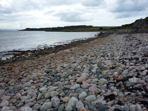
Image of the subsampled Malthi dataset with multiple samples chosen to represent grass and stone.

If you find that you are having a hard time isolating these different features, you may wish to use another metric available through CloudCompare: Roughness. Roughness is calculated based on a point’s deviation from a plane, a plane which is calculated from the position of its nearest neighbours. You define the radius within which its nearest neighbours are calculated with the number you set as the ‘Local Neighborhood Radius’. A very small radius will lend too much weight to micro-topographies of the features captured, and even a tuft of grass may be seen as ‘smooth’ if the planes created by its points and their nearest neighbours do not incorporate enough of the ground surface and become oriented vertically. If your radius is too large, even stone walls will be seen as ‘rough’. Imagine a pebble beach. If you zoom in on a single pebble, its microtopography is quite smooth. If you zoom out further and consider a wider radius, a pebble beach appears quite rough. If we consider the shape of grass compared to stone or ground, grass is ‘rougher’ if we consider a comparatively small surface area, though this distinction will not be visible if we zoom in too closely.

A single pebble; when considering it alone, it appears relatively smooth.

A pebble beach, which appears quite rough because of the scale at which we are viewing it.

Roughness can be calculated by navigating to ‘Tools > Other > Compute Geometric Features’. In the pop-up menu, select ‘Roughness’. The key consideration here is what level the ‘Local Neighbourhood Radius’ should be set to, which may take some experimentation: as explained above, while a segment of the point cloud mostly representing grass would differ substantially in roughness from a segment with the same number of points recording smooth large stones, it is not immediately evident which numeric value this would correspond to. Try zooming in on a patch of grass in the point cloud to fill the screen, until it becomes less distinguishable from its surroundings. Look at the scale in the bottom right hand corner and try setting this as the radius to start.
This will generate a ‘Scalar Field’, which should make it much easier to pick out clear tufts of grass, as ‘rougher’ features will be highlighted in a different colour from its ‘smoother’ surroundings.

Try it yourself! When selecting segments for your classifiers, was it easier to isolate samples before or after calculating roughness? Can you foresee any issues that may arise when applying your classifier to the rest of the dataset?

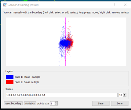
A screenshot of the Grass and Stone samples isolated from the rest of the mesh. The 'merge multiple clouds' button is highlighted with a red box.

In the example above, I have isolated patches of grass (on the right) and segments of wall and stone (on the left). Because the grass is quite sharp and rises vertically quite quickly, I incorporated sharp corners of the walls to ensure that they were not mistaken for grass. The stony walls share more in common with the ground in shape, so it seemed likely that the ground and upstanding structural elements would be classified as the same sort of feature.
- Next, navigate to ‘Plugins > CANUPO > Train Classifier’. In the menu, assign one of your example layers as Class #1 and the other as Class #2. Leave all other options as is, apart from ‘Max core points’. Set this for somewhere between 10,000 and 30,000 (though note that if this is set for more than the points you’ve included in your samples, it will only use the number of points available). Then hit OK.
- Once training has completed, the plugin will display what it has calculated to be the best boundary between the two classifications. This can be altered to create a better visual fit, if needed. Note that the separation between these samples (see below) is not very well defined, so you may want to avoid saving this and try to refine your samples, or save the .prm file and see how it turns out. This is necessary for the next step.

The dialog box displaying the CANUPO classifer - the purple line represents the statistical difference between the grass and wall point clouds.

Ensure that you select the backup of your subsampled cloud so that it is highlighted in the DB tree before this next step.
Navigate to ‘Plugins > CANUPO > Classify’. Select the .prm file you just created as the ‘Classifer file’. The default settings should be sufficient. Click OK.
The point cloud will now have a ‘Scalar Field’ available called ‘CANUPO.class’ that can be visualised. This is how the plugin has classified the entirety of the point cloud – as either ‘Grass/vegetation’ or ‘Stone’ in this example.

Try it yourself! How successful was your classifier at separating the point cloud into vegetation vs non-vegetation geometry?

A visualisation of how CANUPO has classified our Malthi dataset.

The point cloud can then be split according to the classifier by navigating to ‘Edit > Scalar fields > Filter by Value’ and changing this to exclude one of the two classifiers (for example, changing the range to 1.1 – 2.0, which will exclude the Class #1 points). Hit the ‘Split’ button and two separate point clouds will be generated. The ‘Stone-classifier’ point cloud will be retained for meshing.
As we can see above, our classifier was not able to identify all of the grass, and some of Valmin’s later addition to the wall (on the left) was classified incorrectly as ‘grass’.

As you can see above, sometimes the CANUPO plugin will not catch all of the vegetation – you can also use ‘Roughness’ to remove additional vegetation.

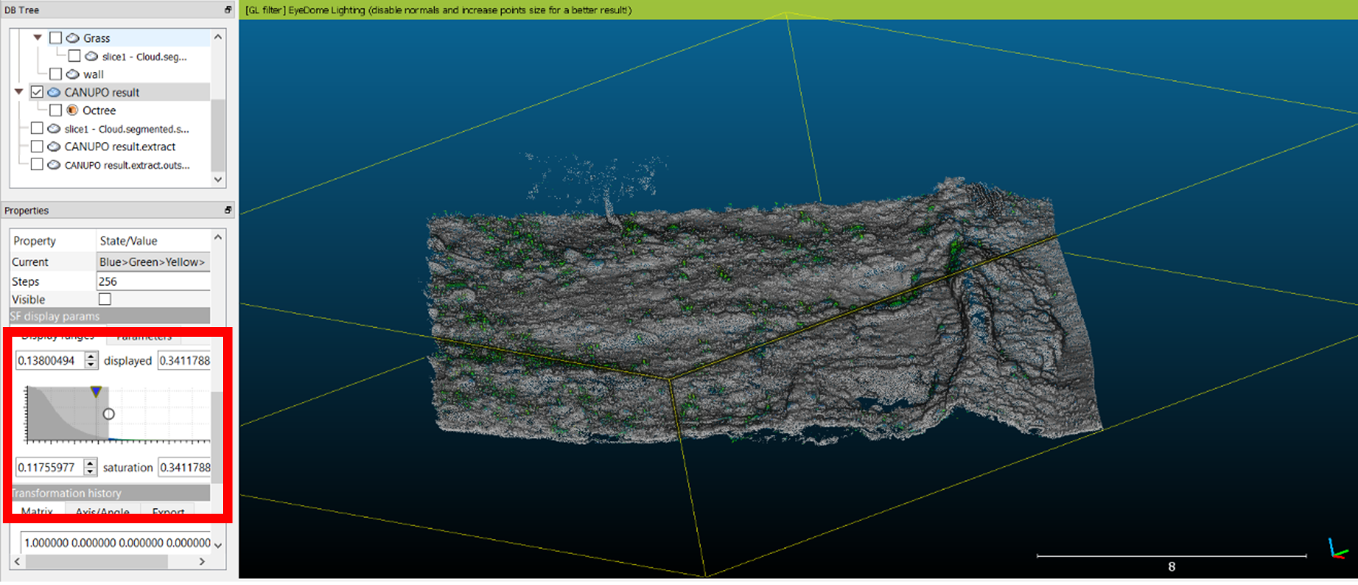
Even if you calculated ‘Roughness’ earlier, recalculate this to generate a Scalar field representing the new range of roughness calculations for this edited point cloud. Examine the point cloud to get a sense of what values/colours have been assigned to the grass patches. Navigate to ‘Edit > Scalar Fields > Histogram’ to get a clearer sense of how the majority of points have been assigned. Under your layer’s ‘Properties’ box, you can also use the histogram under ‘SF display params’ to identify a useful value at which to split your dataset. On the far left of the histogram there is an upside-down triangle that can be clicked, held, and dragged further to the right to better define the difference in roughness between the vegetation of the site and the structures. Once you have isolated the vegetation in a single colour, drag the white dot from the left to ‘gray out’ the data that will be kept. Stop when only the vegetation is left in colour.
Once you have identified where the split should be in your dataset to remove the patches of grass, navigate to ‘Edit > Scalar fields > Filter by Value’ and change the range to reflect your choice (though it should do this automatically). If, as in the example below, the roughness values between 0.11795 and 0.341178 contain most of the vegetation; set the numeric values to reflect this and hit the ‘Split’ button. Retain the non-vegetation point cloud for meshing.

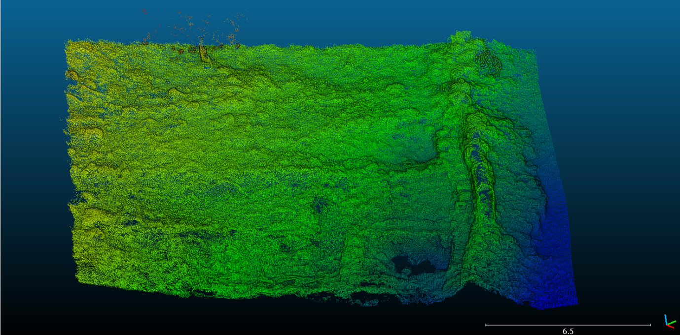
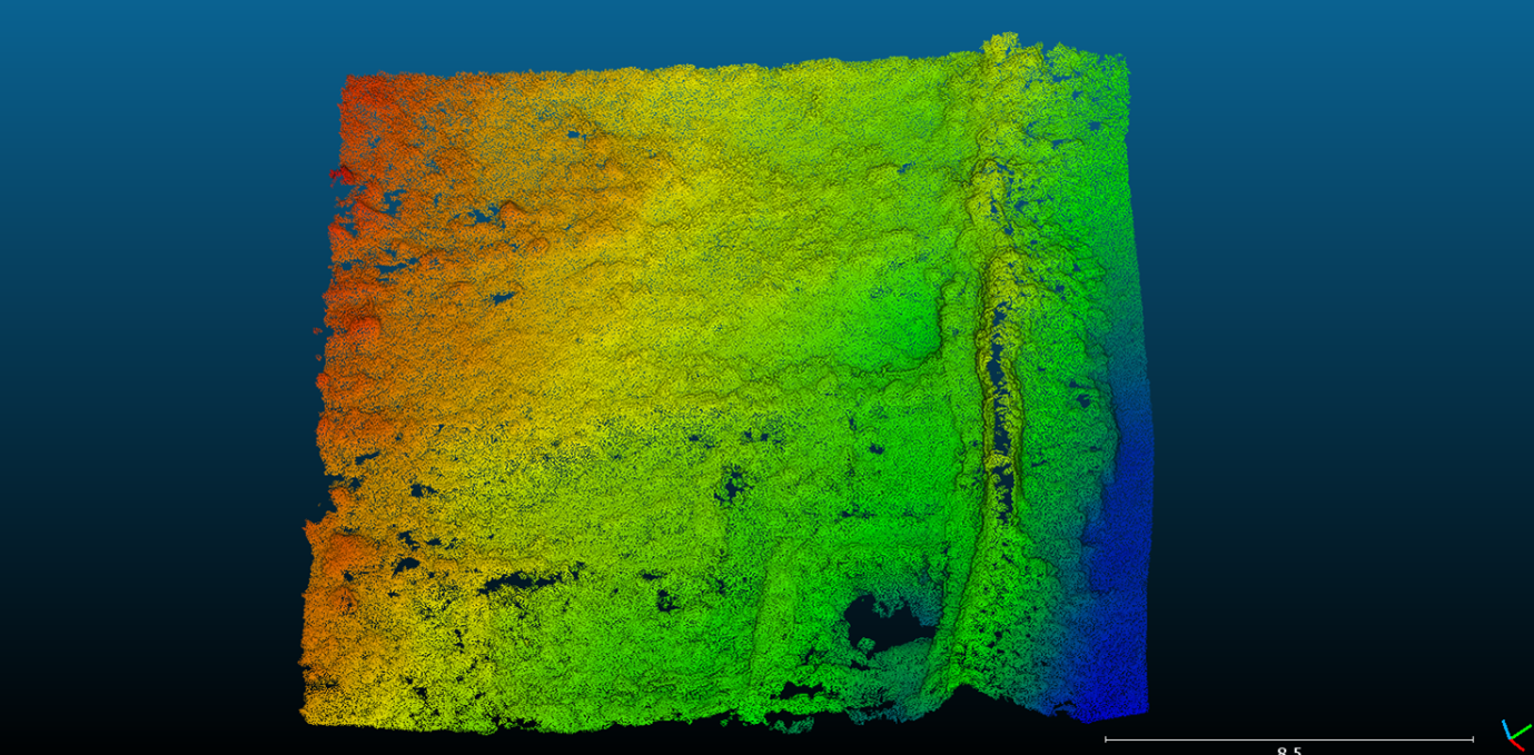
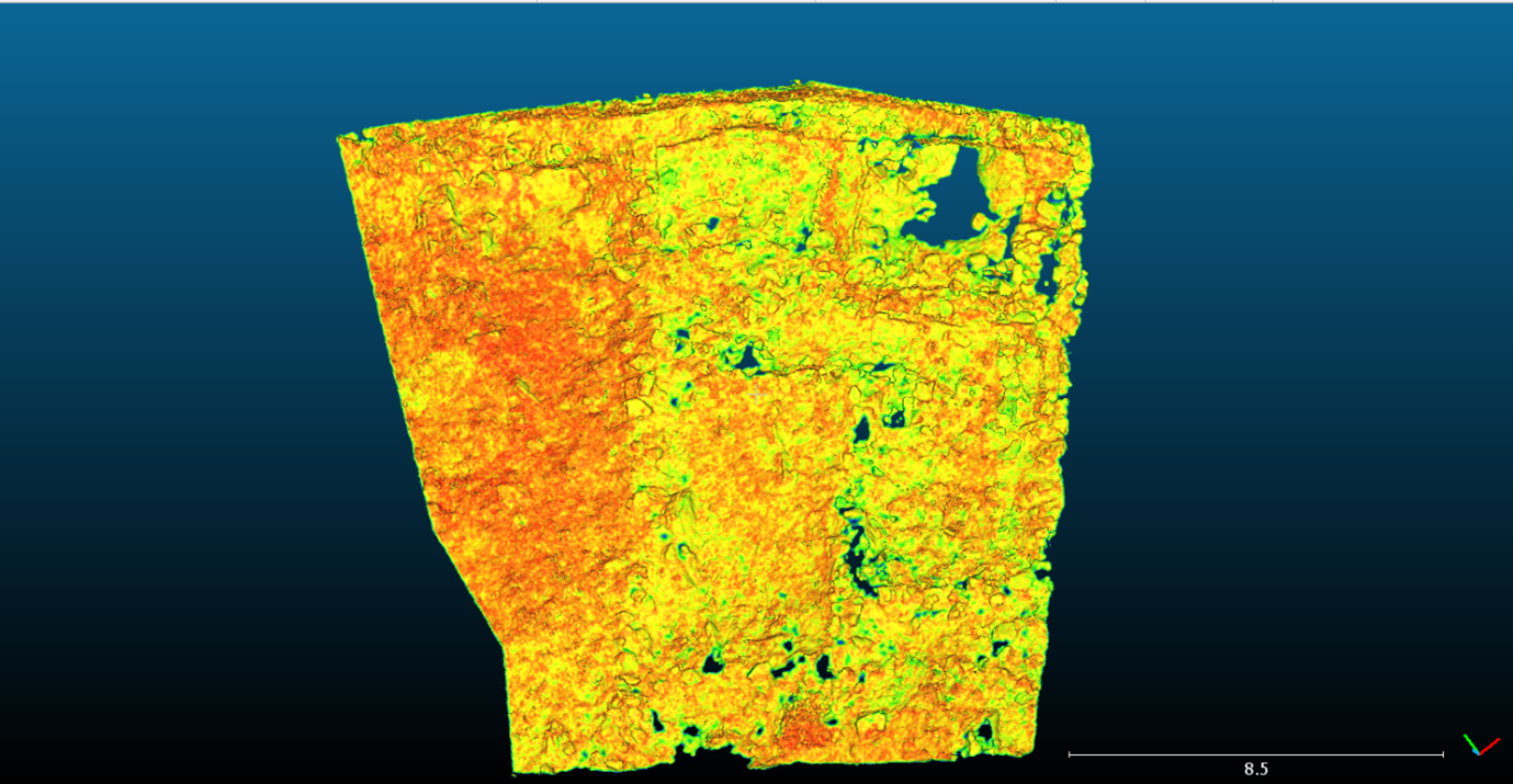
The 'Display Params' histogram has been used to isolate the vegetation from the Malthi data.

Below is an example of the potential results after removing vegetation via CANUPO and using Roughness to remove more vegetation.

The Malthi dataset after using roughness to identify CANUPO samples, creating a CANUPO classifier and removing the vegetation, then applying roughness again to remove further vegetation.

Once you identify your preferred workflow, take special note of this, not only for recording in your paradata, but also because you will need to apply a similar process to the rest of the Malthi dataset to create a full reconstruction of the site.

It is possible that, as you apply the CANUPO classifier from your first dataset to other subsections of the laser scan data, you may find that the classifier wrongly classifies certain features. In the case illustrated below, the CANUPO classifier was defined the northern edge of the site, which is comprised of more open areas and fewer walls than this new subsection, which comes from the centre of Malthi, where structural elements are more densely concentrated.

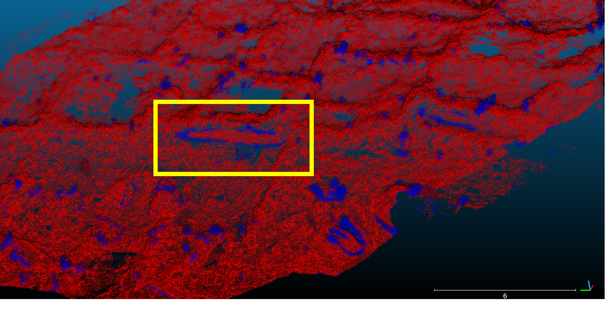
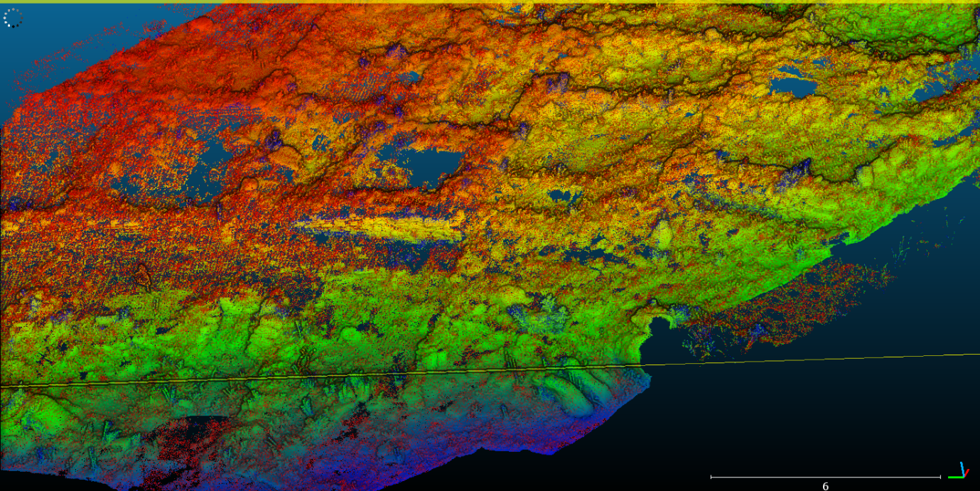
An area of wall from the centre of Malthi (surrounded by a yellow rectangle) has been misidentified as 'vegetation'.

In the image above, part of a wall has been misidentified as vegetation (surrounded by a yellow box; the red mesh represents geometry classified as non-vegetation features, while the blue mesh represents geometry classified as vegetation). We can be certain of this by comparing this subsampled point cloud to the layer containing the full resolution of the original laser scan data for your selection (see image below). If this is the case, you may either want to redefine your CANUPO classifier, or, if it only affects a small proportion of the site, simply remove the incorrectly classified data and append it to the non-vegetation point cloud.

With only the ‘classified-vegetation’ layer highlighted, use the ‘segment’ tool again to isolate these misclassified points. Then, highlight the new layer containing the misclassified points and the layer containing the points that were classified as stone/non-vegetation (use hold CTRL while left-clicking on the second layer in the DB Tree). Navigate to ‘Edit > Merge’ to bring these two datasets together. Repeat as many times as necessary to rectify misclassified points.

The original laser scan data imposed over the sub-sampled and classified data, showing that the points classified as 'vegetation' in the previous image were in fact part of the wall.

After this stage, there will still be some stray points that need to be removed. Some of this may be ‘noise’, or isolated points that appear in scan data but do not correlate to a physical feature in the scene. Vegetation, as we have removed in previous steps, is not the same as noise and would not be removed with the ‘SOR Filter’ or the ‘Noise Filter’. Both of these filters operate under the nearest neighbour statistical principle to identify whether a point is a significant distance from the rest of the dataset based on its distance from the nearest three (or more) points. The Noise filter uses this method to calculate a plane of ‘best-fit’ and removes points that deviate too far from that plane, while the SOR filter rejects points that are determined to be too far from another point based on a number of standard deviations set by the user.

Try using the SOR filter to clean the point cloud by navigating to ‘Tools > Clean > SOR filter’.

Hint
Set the number of points to 15, and set the number of standard deviations to 2. You can try different settings to see how this affects the results.
After running the algorithm, can you tell which points have been removed?

As mentioned above, this will not remove all of the points we may want to remove from the point cloud. The vegetation from the trees may need to be removed – either through utilising the CANUPO system again to create a new classifier, or by removing them manually.

To remove unwanted points manually, align the point cloud so that the points comprising the tree foliage is clearly separated from the ground. Use the ‘Segment’ tool to isolate these points, as you did before. If you are satisfied that you wish to remove these points, delete the tree foliage layer and layers containing other unwanted points from the DB tree.

The final cleaned subsection of the Malthi dataset.

Once you have finished cleaning the point cloud, you should be able to see the outline of the structures much more clearly. Now we need to create a 3D mesh from the point cloud data.

Note that in a real project, now you would save this, go back and treat the rest of your data – you would reuse the pre-trained classifier to remove vegetation from other tiles and reuse your choices for resolution to remove noise. For this exercise, we will continue to the next step.

Step 4: Prepare your data – calculate normals

Before we can generate a mesh from your laser scan data, the next step is to calculate the normals of your points. Normals indicate the directional trend of the surface of your data – not only are they key to building a mesh, as the software needs to know which side of the point cloud is the exterior-facing ‘surface’, but normals also define how ‘light’ interacts with the mesh and affects shading. With a point cloud, because a singular point is not a surface, the software generates a temporary ‘TIN’ mesh (triangulated irregular network) with the points closest to each other; this is used to identify the direction perpendicular to the surface of the TIN mesh, which is recorded as the ‘normal’ of the point.

Compute normals in Cloud Compare
- Edit > Normals > Compute - There are number of options to generate normals in CloudCompare. For this dataset, CloudCompare’s documentation suggests that ‘quadric’ would be best suited, as it describes it as ‘good for very curvy surfaces’. Let the software ‘use octree’ and push the ‘Auto’ button. Use preferred orientation +Z and let it run.

Prepare your data – create a mesh

While there are a number of software packages available that can produce a mesh from point cloud data, we will achieve the best result by producing this in CloudCompare. You can also do this in MeshLab, but we’ll work in CloudCompare.

Step 5: Plan your Meshes

Think and Respond: To keep our datasets manageable, we will need to subdivide the Malthi dataset into smaller chunks for processing, but we will reassemble the site in the reconstruction later. Decide what you will want to have available as a discrete object. Do you want to have individual walls? Walls and surrounding ground? How will you separate buildings that share walls? Whole buildings or sections of the site? Use the published plans of the site layout to plan how these features can be divided. Crop your data appropriately using the segment tool. (Do note that your meshes will maintain their local spatial coordinates, even when exported into different software, so the spatial relationship between two walls that have been saved as different meshes will remain).

Now, make a mesh for each element. Following our ‘test, assess, deploy’ method, pick one or two to work with initially. There is a certain amount of experimentation that is involved in identifying the ideal settings to use when meshing a laser scan, as some will depend on the processing capabilities of your computer.

Navigate to ‘Plugins > Poisson Surface Reconstruction’ (this uses an algorithm proposed by Misha Kazhdan of John Hopkins University)
If you have already computed normals for this point cloud, a pop up window should appear. Set the Octree depth to 11 – setting this relatively high will preserve more detail in the mesh. Note that the highest this can be set is 24, but this will likely cause your computer to crash. Always save your file before trying to mesh your point cloud. You can try this at a couple of different levels to see the difference between the quality of mesh, though there is likely a point at which increasing the octree depth has negligible returns.
Under density, check the box next to ‘output density as SF’. Because the mesh generation algorithm tends to assume the aim is to create a water-tight 3D model with closed geometry, it will be useful to have this checked so that excess mesh can be removed before being exported.

What is a water-tight mesh? This is a mesh that has no ‘holes’, and so is comprised of a single closed surface. There are a number of reasons that a mesh would need to be water-tight: to avoid complications in 3D printing, to allow for certain analyses (like calculating the volume of an object), or to avoid graphical glitches. This is a point of concern in many disciplines that work with 3D objects, so it is not surprising that CloudCompare’s meshing algorithm aims to produce a water-tight mesh.

Under Advanced, try setting ‘Samples per node’ as 1.00 and ‘point weight’ as 1.00.
After clicking OK, it may take some time to produce the mesh, depending on the processing power of your computer.
Turn off the point cloud and inspect the mesh. With the mesh selected in the DB Tree, ensure that ‘Density’ is displaying as the active Scalar field. Scrolling further down in the ‘Properties’ of the mesh, navigate to ‘SF display params’. Drag the small white circle on the left side of the graph towards the right until the empty mesh is no longer visible. Take note of the numbers above the graph. Navigate to ‘Edit > Scalar field(s) > Filter by Value’ and use these numbers to create the desired display range. Hit Split or Export.
If you forgot to uncheck the ‘Preserve Global shift on save’ box at the start of the process, save the mesh as a new file, close CloudCompare, and re-open the mesh. You will again be prompted whether you want to ‘Preserve the global shift when saving’ – make sure this box is unchecked, then resave your mesh. This will prevent any issues when analysing the mesh in other software, including MeshLab and Blender.

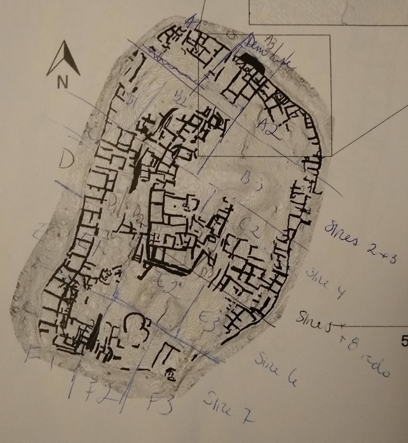
The cluster of structures from our original point cloud have been meshed in this image.

Despite removing the global coordinates, the meshes produced from the Malthi laser scan data will still retain their spatial relationships to each other when exported (as long as you have ensured that the same ‘global shift’ numbers have been applied when importing each dataset). Sub-setting or tiling your dataset is a standard approach to landscape-scale or site-scale 3D datasets. The process does require planning, however, so ensure that your tiled datasets are clearly labelled and correlate to either a digital or physical plan of the site. This will help you catch any errors in orientation or coordinates that might occur in later steps. Below is an example of how the dataset can be divided into tiles (labelled A1-F3). Be sure that these are named in a planned, sensible way to make it easier to piece together in later Exercises.

An example of how you can subdivide the Malthi site dataset - ensure that you name these tiles in sensible ways to make piecing it together easy in later exercises!

n.b. In a real project, you would now go back and deploy this routine over all your point clouds you want to convert to meshes.

Think and Respond: By the end of this process, you should have a mesh of all or part of the site of Malthi. Take a closer look at the mesh – is this a sufficient level of detail for what you will need to reconstruct the site? What essential parts are present, if the aim of the reconstruction is to get a sense of how the site would be navigated? Which essential parts are missing? Are there any stray bits of mesh that need to be cleaned up/removed?

Step 6: Export your data

Ensure that, at a minimum, you have saved your completed mesh(es) and their associated point cloud as a backup .bin file in case you ever wish to make adjustments. As noted above, you may want to use the map from the preliminary Malthi report to record the names you gave subsets of the data.

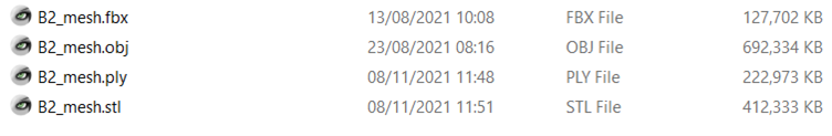
To export your data, all you need to do is highlight the mesh you wish to export in the DB Tree and hit the ‘Save’ icon. The dialog box will provide a number of file format options, but we need to consider which will be accepted by the software we will use in later steps. Most 3D modelling software packages will work with .obj, .ply, .stl, and .fbx file types. If we had colour or texture data to export, this may have impacted our decision (.stl files will not save colour or textures, .ply files can only maintain a single texture file, .obj files can occasionally become disassociated, as we saw with the photogrammetric models before, and .fbx files will usually save colour, normals, and textures because they are often used in animation projects). However, our biggest concern at the moment will be the file size of the object, as we will be assembling a substantial number of models in a single file.

Try saving one of your meshes in the .obj, .ply, .stl, and .fbx file types. Take note of the size of each file in the file explorer window. Which is the smallest file size? However, we also need to take archival standards into account – generally, digital archives will prefer either .obj or .stl formats as they are simple formats and well-established, so almost all 3D software will accommodate them. Though we will likely be working with .fbx files in later exercises, we’ll need .obj files to do some additional processing before we can piece our reconstruction together. So, be sure to export your meshes as .obj files twice – once so that we have a pristine copy for the later archival stages of your project, and one to work with in other software through the next steps. Consistency is key, as sometimes different file types will import into software in different ways (.obj files will import into Blender rotated at a 90˚ angle, for instance, while .ply files will not rotate them).

The files generated by exporting one of each file type from tile B2. The FBX file is 127 MB, the OBJ is 692 MB, the PLY is 222 MB, and the STL is 412MB.

Once you have saved your files with sensible names in formats suited to their intended use, be sure that your data is organised in a clear way. If you have files that you intend to use in the reconstruction, save them in a folder that indicates that purpose. If you have files that have been saved for the archive, put these in a separate folder. Often, moving files into new folders after they have been used in other software (like Blender) will cause directory issues, so it’s best to keep them in one place for the course of the project.

Well done! You now have the shapes of the walls, and they are georeferenced. This is what you would need for a reconstruction that helps you to think through movement around the site.

In addition to the information from the archive, there are a number of other resources with which you may want to familiarise yourself.

What other information is available?

Valmin’s report on the 1920s-30s excavations (if you can find a copy in the library)
Malthi interim report from Lindblom and Worsham on the work carried out between 2015-2016, with new thoughts on the old interpretations from excavations in the 1920s-30s: http://ecsi.se/opathrom-11-02/
Worsham’s report on scan results: https://sparc.cast.uark.edu/assets/final_reports/Worsham_SPARC_Final_Report.pdf
Two 3D models produced through aerial photogrammetry in later field seasons have been uploaded to Sketchfab by the Malthi crew: one is focused on the site, while the other provides additional landscape context. Though the detail contained in the meshes are much lower than what you have just produced, they do provide a coloured texture that we may want to utilise in our rendering.

Think and Respond: At this point, you should be able to fill out a good deal of your Design Document, including the Project Brief, Overview, Project Aims, many of the Resources, and some of the Constraints. Review your previous ‘Read and Respond’ answers for ideas!

Resources for Exercise 1:

Directly cited:

Archaeology Data Service. 2021. Guidelines for Depositors: Downloads (Vers 4.1). URL: https://archaeologydataservice.ac.uk/advice/Downloads.xhtml.
Brodu, N. and Lague, D. 2012. 3D Terrestrial lidar data classification of complex natural scenes using a multi-scale dimensionality criterion: applications in geomorphology. ISPRS Journal of Photogrammetry and Remote Sensing, 68 (March 2012): 121-134.
Boardman, C. 2018. 3D Laser Scanning for Heritage: Advice and Guidance on the Use of Laser Scanning in Archaeology and Architecture. Swindon. Historic England.
Denard, H. 2009. The London Charter for the Computer-Based Visualisation of Cultural Heritage, draft 2.1. http://www.londoncharter.org.
George Drettakis, Maria Roussou, Alex Reche, Nicolas Tsingos. 2007. Design and Evaluation of a Real-World Virtual Environment for Architecture and Urban Planning. Presence: Teleoperators and Virtual Environments 16(3): 1-21.
Forte, M. 2014. Virtual Reality, Cyberarchaeology, Teleimmersive Archaeology. In (eds) Remondino, F. and Campana, S. 3D Recording and Modelling in Archaeology and Cultural Heritage Theory and best practices. Oxford: Archaeopress. Pages 113-127.
Jeffrey, S. 2015. Challenging Heritage Visualisation: Beauty, Aura and Democratisation. Open Archaeology, 1(1): 144-152. https://doi.org/10.1515/opar-2015-0008.
Pujol Tost, L. 2008. Does Virtual Archaeology Exist? In: Posluschny, A., K. Lambers and I. Herzog (eds.) Layers of Perception. Proceedings of the 35th International Conference on Computer Applications and Quantitative Methods in Archaeology (CAA), Berlin, Germany, April 2–6, 2007 (Kolloquien zur Vor- und Frühgeschichte, Vol. 10). Dr. Rudolf Habelt GmbH, Bonn, pp. 101-107.
Lanjouw, T. 2016. Discussing the obvious or defending the contested: why are we still discussing the ‘scientific value’ of 3D applications in archaeology? In: (eds) Kamermans, H., de Neef, W., Piccoli, C., Posluschny, A., and Scopigno, R. The Three Dimensions of Archaeology: Proceedings of the XVII UISPP World Congress (1–7 September 2014, Burgos, Spain). Oxford: Archaeopress. Pages 1-12.
Watterson, A. 2015. Beyond Digital Dwelling: Re-thinking Interpretive Visualisation in Archaeology. Open Archaeology, 1(1): 119-130. https://doi.org/10.1515/opar-2015-0006.
Wilhelmson, H. and Dell’Unto, N. 2015. Virtual Taphonomy: A New Method Integrating Excavation and Postprocessing in an Archaeological Context. American Journal of Physical Anthropology, 157: 305–321.
Worsham, R., Lindblom, M., and Zikidi, C. 2018. Preliminary report of the Malthi Archaeological Project, 2015–2016. Opuscula, 11: 7-28.