Exercise 1

Part B: Get to know your data - start by reading the metadata and reports

With any sort of dataset, we need to assess the quality of the data. There are a number of considerations to take into account when assessing the 3D datasets you have at your disposal. The first step is to obtain any reports or metadata concerning the dataset. Metadata is information that describes other data – this may describe something as simple as the file format in which the data is saved, what equipment was used to record the data, or what other files are associated with the data. Understanding your data is essential as there are several characteristics that will dictate which software packages will be most useful in managing and processing the dataset for use.

Reading and Understanding the Metadata Report

• This exercise assumes you know a bit about terrestrial laser scanning. If you need a refresher on how terrestrial laser scanning captures 3D data, we highly recommend that you review English Heritage’s guide ‘3D Laser Scanning for Heritage’.
• Metadata is usually recorded in a text-based format or a spreadsheet, depending on the requirements of the archive. Download a blank template for Laser Scan metadata from the Archaeology Data Service from this link. Compare the requirements for the ADS template to the Malthi metadata report – are there any differences? Why might this be?
• For Malthi, the metadata report can be found at https://doi.org/10.5281/zenodo.3826550; download the file Malthi2015_Report.docx. This provides all of the metadata for the initial data capture, including:
  • Basic project information, including the survey creators (see Project Overview in Malthi2015_Report),
  • the research motivations for recording the site in this way (summarised in Project Overview in Malthi2015_Report),
  • the type of scanner used (Leica C10 Scanner),
  • the number of scan positions (78), the coverage of the scanner (within the fortification wall), and scanner resolution (the space between points: 0.01m x 0.01m at 20m from the scanner, 360x90 degree FOV around each),
  • that there is no real-world colour associated with the dataset,
  • how the scans were aligned and what software was used (visually aligned and then registered, Leica Cyclone 9.0),
  • how the dataset was georeferenced (georeferenced sane points on standing architecture directly to the DGPS survey data),
  • Global Registration Error (0.019 m),
  • the file types that were originally generated (.pts ascii files),
  • the file format(s) in which the dataset has been saved/archived (.las, .laz, .lasd, .imp, .bin). Some of these file types may be unfamiliar to you – these 3D files are commonly used in geospatial analysis; a list of these can be found here. (Other file types we will be discussing later are considered ‘3D graphics file types’, a list of which can bre found here.) .las and .laz file types are standard file types for laser scanning data. .laz is the compressed (like a zip file) format for a .las file. (To read more about .las files, refer to the ASPRS’s page here.),
  • and the type of data these files contain (point cloud). A point cloud is composed of calculated points in three-dimensional space, produced when a digital imaging technique measures and records the surface of an object; each point is defined by a set of coordinates on the X, Y and Z planes.

Think and Respond: Summarise what you now know about the dataset after reading the metadata report. What are some of the challenges you can see in working with this dataset? Take note of what you think is most important and add it to your Design Document under the Resources: Available section.

Get to know your data – open and visually review samples

A step-by-step guide from this point onward in Exercise 1 can be found here.

Now that we know what type of data and what format the files are saved in, we need to identify how much of the site is represented in the record. First, we need to open the dataset in software well-suited to dealing with point clouds in the .las or .laz format. There are a number of paid software packages that will work with these files (Leica Cyclone, Autodesk ReCap, Esri ArcGIS), but there are a number of free and reliable open source software packages available. In this case, download and install the relevant version of CloudCompare.

• Next, download the Profile slices from the relevant Zenodo entry from the SPARC archive here: https://doi.org/10.5281/zenodo.3833880.
• Unzip the .zip file to a new folder.
• Examine the files in the file explorer window. Ensure that ‘Size’ is visible. You may notice that the file sizes are quite large. If we look at Slice1.las, we can see that it is about 4 GB in size. While the corresponding .laz files are smaller, remember that these contain the same data as the .las files, the data is simply zipped into a compressed file format. When it is opened, it will still contain the same amount of data as the .las files. Unless you have a computer with significant processing power, you will not be able to open more than four or five of these at a time without the software crashing. Let’s open one file at a time.
• In CloudCompare, navigate to ‘File > Open >’ And choose your first profile slice.
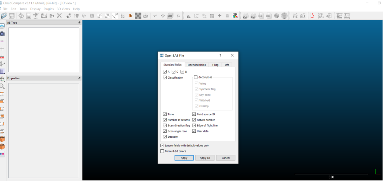
• This will prompt a pop up dialog box, where it will ask you which information fields it should look for in the file and let you know how many points are in the file (under info). Leave the default settings as they are and hit ‘Apply’.

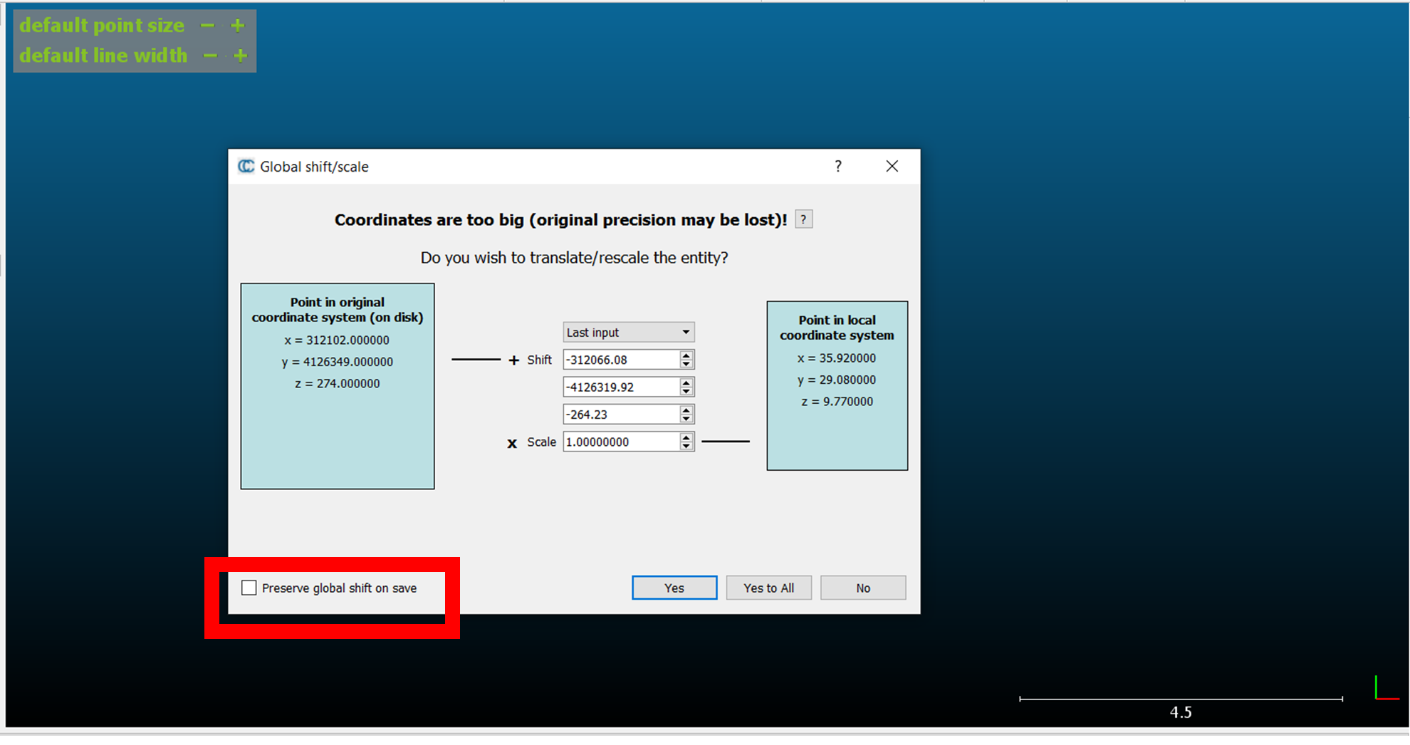
• This will prompt a new dialog box to appear. The software wants to shift the dataset to the local coordinate system (closer to 0, 0, 0) because the data’s current coordinates correspond to the site’s global position using UTM (Universal Transverse Mercator) coordinates, which indicate the site’s distance from the equator and the prime meridian in metres. These coordinates are quite large and, while this is common practice in software designed to work with the geospatial sector, like ArcGIS, most 3D modelling software is not designed to work with such large numbers. If we keep the original coordinates, some 3D modelling software will place the dataset 4 million units away from the origin; in other software, like MeshLab or Blender, keeping the UTM coordinates can also cause graphical glitches. Because we will not be using this data in geospatial software, we need to make sure that the UTM coordinates are not preserved.
  • Ensure that the box that says ‘Preserve Global shift on Save’ is unchecked.
  • Take note of the numbers used in the proposed shift for your records to ensure that the same translation is applied to the other profile slices in the future. Otherwise these will be misaligned in later steps.
  • Allow CloudCompare to translate the dataset to local coordinates with the recommended settings.

• After some time processing, a cloud of white points should appear. To better define the features in the visualisation, there are a couple of options.
  • You can apply shaders – navigate to Display> Shaders & Filters> and select EDL.
  • To add a height map, with the ‘slice 1 – Cloud’ point cloud data highlighted in the DB Tree window, navigate to ‘Edit > Export coordinate(s) to SF’. When the dialog box appears, ensure that ‘Z values’ are checked before hitting OK. This has converted the ‘Z coordinates’ or ‘height values’ of your points to a Scalar field, which is visualised with a rainbow gradient by default.
  • Explore the rest of the laser scan datasets – left click and drag anywhere in the viewer to rotate the scan data. Right click and drag will pan the dataset. Use the scroll wheel on your mouse or the + and = buttons on your keyboard to zoom in and out.

We should also explore the other 3D datasets available in this archive to see if they will be useful in our reconstruction. Download MeshLab (or use CloudCompare to open the mesh, but note that the colour will not be applied). On Zenodo, search for Malthi SfM – this will come up with the Structure from Motion photogrammetry records produced in 2015 to create detailed 3D models of two wall segments at the site. Photogrammetry is a different method of 3D data capture which involves taking overlapping photographs of an object or structure, which software then uses to build the 3D geometry of the feature or object.

• Download the files in the Malthi2015_SfM_ProcessedOutputs and open them in MeshLab. (If the textures do not automatically apply themselves, navigate to ‘Filters > Texture > Set Texture’ and choose the corresponding .jpg file).
• Flip this right-side up by left-clicking and dragging across the screen. If we examine this dataset, it is not clear which walls these represent from the provided metadata. If we import both walls into the same MeshLab project, one is significantly smaller than the other, which leads us to wonder if both were scaled accurately. While these are textured and could be useful references if trying to create a photorealistic appearance for our reconstruction, the lack of context and certainty regarding their scale makes it very unlikely that we will utilize these meshes in the reconstruction itself, especially when the laser scan data has far more coverage.

Think and Respond: Now that you have viewed the different point clouds and meshes available to you, assess how much of the data is needed for your reconstruction. What do you notice about what was captured in the scan data? How much of the site has been recorded? According to the report, everything within the fortified wall was recorded, though there may be related structures situated outside of this boundary. Will the trees and grass captured in the laser scans help or impede your reconstruction? It seems unlikely that an occupied settlement would have been covered in grass, so we can plan to remove these later. What level of detail will you require for your reconstruction – will the outline of buildings be sufficient to build from? While the snapshots of the full-resolution point cloud in the report show that the laser scans have recorded individual stones quite clearly, you need to decide if that level of detail is necessary for what you need to achieve. To meet this design brief, do you need the entire dataset, or only subsections of the recorded data (ie one house)? What size of dataset will be easy to work with (considering your computer’s hardware; if you find you are having issues with this, you may need to use one of the computers in UofG’s Digital Archaeology lab)? Do you need meshes or points? While point clouds appear quite attractive, the software we will be using and games engines [i.e. 3D modelling software which will be further discussed in later Exercises, and Unity and Unreal engines] are not generally designed to work with point clouds in this way. Summarise and incorporate your thoughts on these considerations in your Design Document template, particularly in the ‘Resources’ and ‘Constraints’ sections.

Back to Exercise 1 Part A

Continue To Exercise 1 Part C