Exercise 3

Allow at least 1 1/2 hours for Exercise 3 - additional time will be needed if creating Normal maps for multiple regions of the laser scan data from Malthi.

Optimising Reality-Captured Assets in MeshLab and Blender

Part A: Cleaning and Decimating

So far, you have done a lot of preparation for your archaeological reconstruction. In Exercise 1, you took archived point cloud data from laser scans and processed this into a series of cleaned, georeferenced meshes that we will be using as the foundation for the 3D reconstruction. In Exercise 2, you made key design decisions about the reconstruction, including what the structures should look like (shape, materials, etc) based on the archaeological evidence, how to set aims and goals with collaborators, and what software you will be using to put together the reconstruction based on your budget, skillset, and needs to create the reconstruction.

The preparation does not end here, however. There is a certain amount of additional cleaning that will need to be completed, for which we will use MeshLab. We will then decimate the meshes in a software called Instant Meshes. Finally, we will import both the cleaned high-resolution mesh and the decimated mesh into Blender to ‘bake’ or ‘paint’ the detail from our high-resolution mesh onto the low-resolution mesh so that all components of our foundation can be brought into the same Blender project.

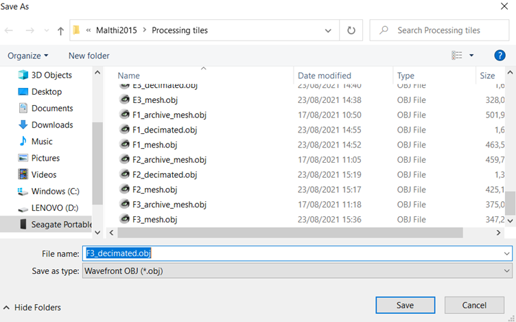
Note: Before we begin these next steps, decide how you will be naming your meshes to ensure consistency. You should already have your meshes relatively organised and clearly named, including one mesh reserved for archiving later on (perhaps named ‘A1_Malthi_archive_mesh.obj’ or ‘A1_archive_mesh.obj’) and one ready to be cleaned (named ‘A1_mesh.obj’ or something similar). We will, at the very least, be producing a decimated mesh and a low-resolution mesh with an associated normal map (in an image file) by the end of this exercise, so it is recommended that you decide how you will be naming and structuring these files. If our final aim is to bring several meshes into a single Blender file, it is important to have a clear structure from the beginning – if you move these meshes or image files after putting all of your meshes together to create the foundation, these will become disassociated and will need to be reconnected in Blender manually. To avoid having to do this for each mesh later in the process, stick to a structure!

MeshLab Cleaning

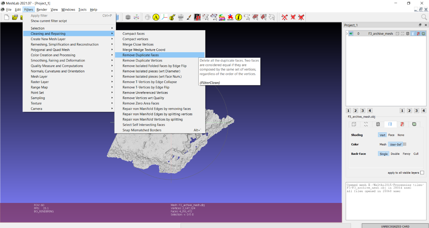
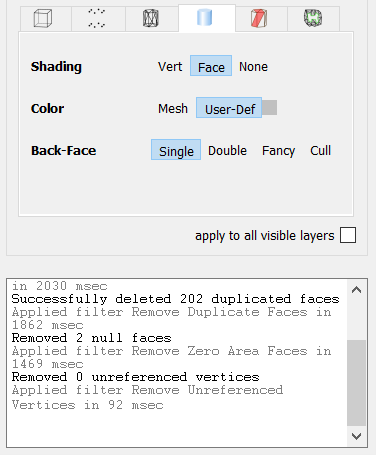
Pick the part of the site that you are most interested in reconstructing for this exercise. To prepare our foundation for the reconstruction process, there is a certain amount of mesh cleaning that needs to be done. The following workflow largely borrows from that suggested by Mister P., who has produced a number of incredibly useful MeshLab tutorials, including this one about cleaning meshes. Now that we have meshes to work with, we can use the powerful tools housed in MeshLab software to prepare the dataset further. First, there are a number of filters that we should apply to ensure that the meshing process did not introduce any issues that need repair. Under ‘Filters > Cleaning and Repairing’, select ‘Remove duplicate faces’. Next, navigate to the same menu and select ‘Remove duplicate vertices’. Not only are these duplicates unnecessary and increase the file size of the mesh, but double vertices and faces can have a negative impact on the appearance of shading in later stages of the project. From the same menu, run ‘Remove Zero Area Faces’ and ‘Remove Unreferenced Vertices’. Both of these can affect the appearance of normals and textures. Finally, it is advised to ‘Filter > Selection > Select Non Manifold Edges’, clicking apply to highlight them, and to delete these by clicking ‘Delete Selected Faces and Vertices’, as these will affect your ability to run certain algorithms in Meshlab, including ‘Close Holes’, which we will be running later. As each process runs, the bottom right corner of the ‘Layer Dialog’ will indicate the results of each.

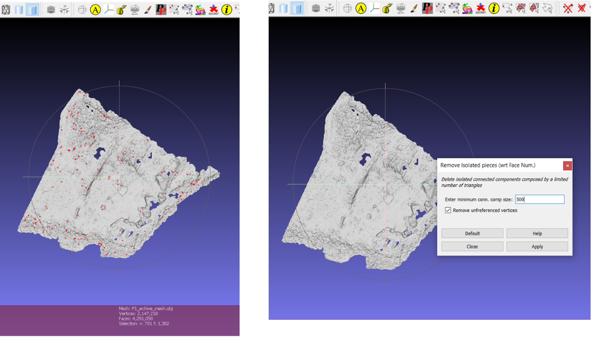
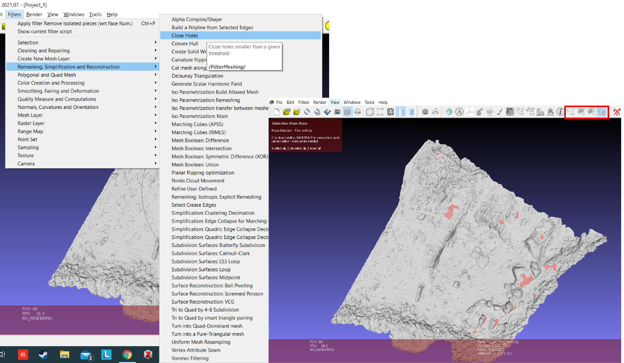
When examining your mesh at this point, it is apparent that some stray points have been meshed into individual faces or small irregular meshes just above the ground surface. This is quite difficult to remove manually, so we will be using one of the filters in MeshLab, ‘Filters > Cleaning and Repairing > Remove Isolated Pieces (wrt Diameter)’ or ‘Remove Isolated Pieces (wrt Face Num.)’. Because we only want the mesh of the ground surface, which should not have any isolated pieces, the automatic settings for the wrt Diameter function will work. Alternatively, if using the wrt Face Num. function, we can set this relatively high as we know the mesh itself is composed of millions of faces. If we set this at 500, this should remove any problematic pieces without causing any issues for our mesh. Finally, in the ‘Filters > Remeshing, Simplification, and Reconstruction’ menu, select ‘Close Holes’ and apply. If you wish to see where the holes have been filled, ensure that ‘Select the newly created faces’ box is checked. Just be sure that, before you export, you select the any of the selection tools and hit ‘D’ to ‘Deselect all’, or the selected mesh will be a different colour in your exported mesh.

Note: While most 3D modelling software packages will have some sort of ‘fill hole’ function, they will be based on different algorithms, and so some are more effective in some situations than others. If we had a large hole caused by the position of the laser station on our site, for example, it may be more effective to fill the hole with CloudCompare’s meshing algorithm, as it seems to cope better with filling large holes (likely because it has the original point cloud to refer to). MeshLab’s algorithm will neatly fill most small holes, including those that are not immediately obvious. Blender’s ‘fill hole’ algorithm will not always identify small holes, and so is better suited to manually filling holes on decimated meshes.

You may wish to trim your mesh, as wavy edges can cause issues in the next steps. Use the ‘Select Faces/Vertices inside polyline area’ tool (in the red box in the image below, or use the search function to find the tool by clicking on the magnifying glass in the top right corner). When you have surrounded the mesh you wish to remove with the polygon, tap ‘Q’ to Select the mesh and use the ‘Delete Selected Faces and Vertices’ tool again (in the blue box below) to remove them.

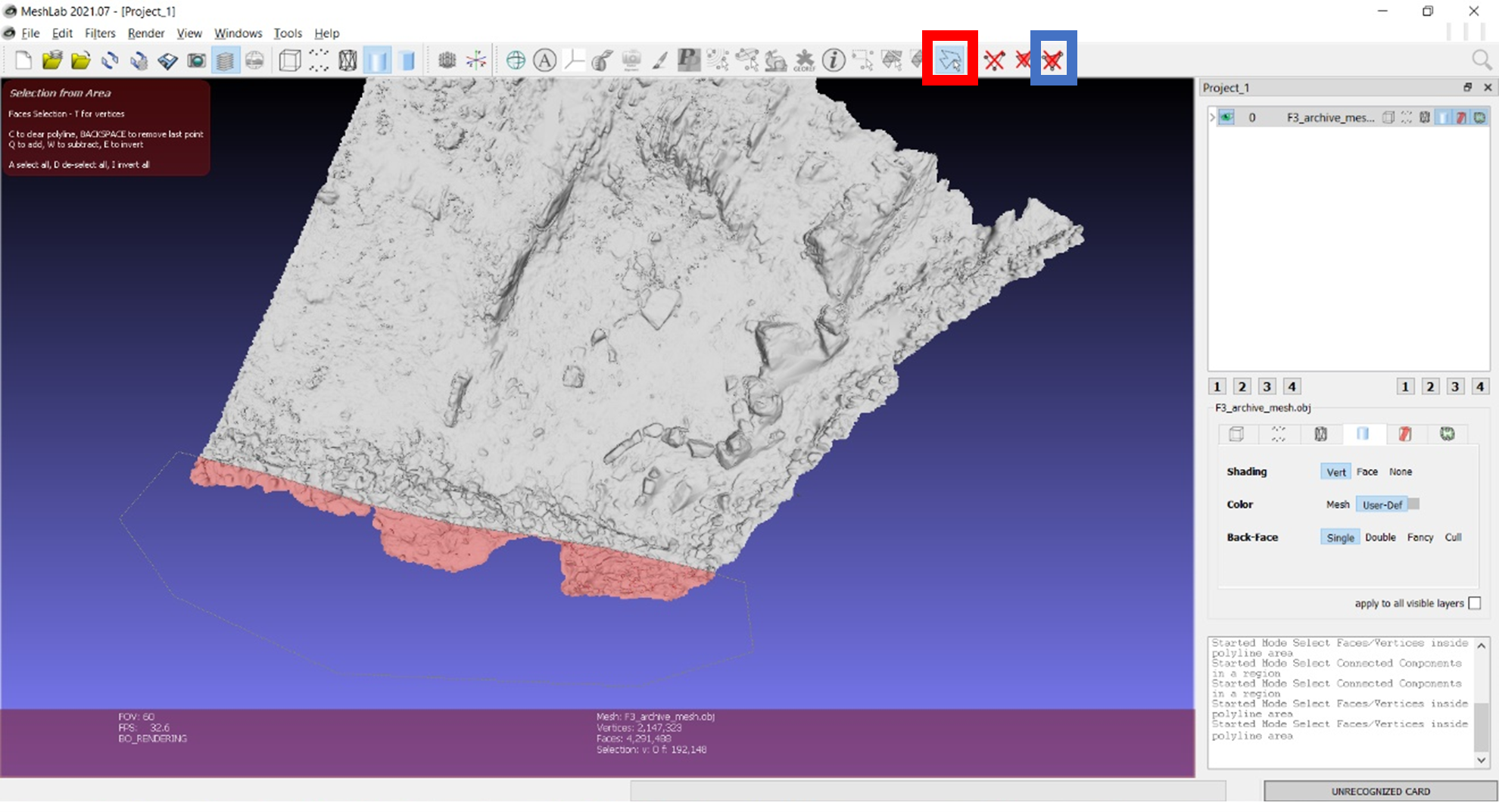
If you are happy with how your mesh appears, you can now navigate to ‘File > Export Mesh As’ and give it a new name or ‘Export Mesh’ if you want to save over your original file. Export it as an .obj file.

Think and Respond: Does your mesh look significantly different after this clean-up process, or were most of the changes invisible to you? Do you think this is still a metrically-accurate mesh? Are there any other features you may want to remove at this stage (rubble piles from early excavations that would not have appeared this way in the Bronze Age)? Does this mesh still represent the archaeological reality of the site?

Import mesh into Instant Meshes

A step-by-step video for this point onward can be found here.

Ensure that you have installed Instant Meshes before importing your cleaned mesh into the software. The purpose of this software is two-fold: 1) To rapidly create a decimated version of your highly detailed meshes, where you control the number of vertices and can quickly recalculate a new decimated version if not enough detail is preserved, and 2) to convert your triangulated mesh into a quad-based mesh. (Note: As you may surmise from our ‘Software choice’ activity in Exercise 2, this is undoubtedly only one of many software options available that will offer this functionality, but this is one that is free, works well, and does not take too much space on your hard drive.)

Why Quads? As we noted a difference in how geospatial specialists work with 3D data from most other 3D specialists in Exercise 1, there is also a difference in how those who work with reality-captured data compared to those who create their own 3D meshes from scratch. In the latter group, most 3D artists prefer working with quads instead of triangles, as they are easier to work with (this is a complex topic that you can search for online; if you would like to do a deep-dive you can start here) and often produces better results for animation. As such, many 3D software modelling packages have developed to prioritise quads; many of Blender’s functions, including the ‘subdivision’ function, which we will use later, work best with quads.

To import your high-resolution meshes into Instant Meshes, click the ‘Open Mesh’ button in the top left corner. You will want to leave ‘Remesh as’ set to ‘Quads’. One important option to enable is ‘Align to Boundaries’ under ‘Configuration details’. If the decimated mesh is larger or covers more area than the original, high resolution mesh, this can cause graphical glitches when normal mapping. Set the target vertices count quite low; you may want to start with 3K or 4K. Next, click the ‘Solve’ button under ‘Orientation field’ and, once that is finished, for ‘Position field’. Once these have completed, click ‘Export Mesh’, enable ‘Pure quad mesh’, and set Smoothing iterations to 1. Then click ‘Extract Mesh’.

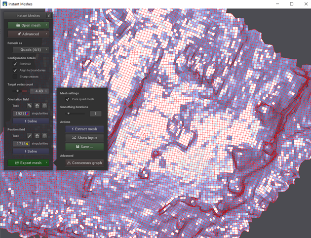
After the decimated mesh has been extracted, the software will automatically switch from the original mesh to the decimated. You can view your original mesh by clicking the ‘show input’ button. Ensure that enough detail is preserved in the decimated mesh. But how much is enough detail?

Normal mapping is essentially painting the ‘detail’ onto the mesh – so for the decimation step you really need to consider how much of the original geometric shape you want to preserve. When creating the normal map, we will essentially be creating an image of a very detailed plan map from the difference between the detailed mesh and the simplified/decimated mesh – which can then be ‘painted’ onto the decimated mesh. So if you want to keep the walls that are about 1m high, you need to make sure your decimated mesh retains that shape. If on the other hand, you want the basic elevation information and a detailed plan image, you can opt for fewer vertices.

Note: There are other issues to take into account, as you will see in Exercise 5 – there are often file size restrictions in certain types of outputs, including Sketchfab and Unity. Be sure that you take this into account at this stage; if the final composite mesh needs significantly more decimation after you have already generated Normal Maps, it may cause tearing in the maps.

Try it yourself! Try processing your original mesh into decimated meshes with different counts of vertices. Which level seems to preserve enough detail, in your opinion? How many meshes have you broken the Malthi dataset into? Do you think the file size of the decimated composite dataset be small enough to work with easily?

When you are happy with your decimated mesh, you can click the ‘Export’ button. Be sure that when you give your decimated mesh a new file name that you type in the file extension at the end – otherwise it will not export the decimated mesh.

Back to Exercise 2

To Exercise 3 Part B