Exercise 4: Quantitative Approaches to Interpretation

(Allow at least 1 hour for Exercise 4)

A step-by-step video guide to Exercise 4 can be found here.

As demonstrated above, the use of morphometric parameters as Scalar Fields has a great deal of potential for quantitative analysis. In this exercise, you will learn to:

• Use CloudCompare to calculate morphometric parameters and visualise these as Scalar fields;

• Work with multiple meshes at the same time by assigning individual meshes to different 3D Viewports;

• Incorporate quantitative approaches into an interpretation of the lifeway of PH 25.

In Exercise 2, we examined the potsherd PH 25 in Meshlab; we used visual inspection and simple measurements to hypothesise how the fingerprints were applied to the potsherd, and we considered whether all of these fingerprints could have been applied as a part of the same ‘event’. Let’s hypothesise that some of these fingerprints were added at different times, or even during different manufacturing stages. Perhaps the clay was wet and had not had time to dry when some of these fingerprints were made – this would have made the clay more malleable, and so the fingerprints may have made more of an impression, or more clay may have come away with the potter’s finger as a result. We could then hypothesise that fingerprints made at this pre-drying stage would have resulted in rougher fingerprints than those made after the pot had dried. To test this, we could compare the average roughness of each individual fingerprint in CloudCompare.

1. First, import the .stl file for PH 25 into CloudCompare. Use the Segmenting tool to isolate the fingerprints you identified in Exercise 2 into separate meshes. Be sure to Rename these parts in a memorable way (in the following steps, they have been labelled as M0, M1, M2, M3 and M7, corresponding to their measurement labels in Exercise 2). Continue to segment the fingerprints from the .Remaining mesh. Ensure that these individual meshes are clipped as close to the edge of the identifiable fingerprint as possible.

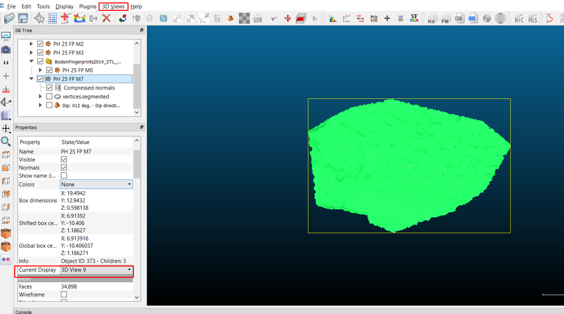
2. If you want to allocate these 3D models to different 3D spaces, you can do this with the ‘3D Views’ drop down menu. First, create a new 3D View. Then highlight one of the meshes in your DB tree. Under its ‘Properties’, you can change its ‘Current display’ to the new 3D View window. The relevant menus are highlighted in the image below.

1. After you have each of the individual fingerprints isolated on different 3D Views, ensure these meshes are uniformly flat as we did in Exercise 3.

   a. Use the ‘Plane’ option from the ‘Edit’ dropdown menu and choose ‘Fit’.

   b. Copy the Transformation Matrix, ensure the Mesh you wish to align is highlighted in the DB Tree, and paste the matrix into the ‘Apply Transformation’ pop up window.

   c. Then, export the newly aligned Z coordinates using the ‘Export Coordinates to SF’ option under Edit > Scalar Fields. Repeat this for each of the fingerprints.

2. As briefly explained at the start of Exercise 3, some of the functions of CloudCompare work with the vertices of the mesh as a point cloud. This is the case for calculating roughness, surface variation, and other morphometric parameters. These individual points comprising the point cloud are the only ‘real’ measured data in a 3D mesh, as they are the points that were actually measured and recorded during data capture; the mesh is a rough approximation of the object’s surface based on the density of the point cloud.

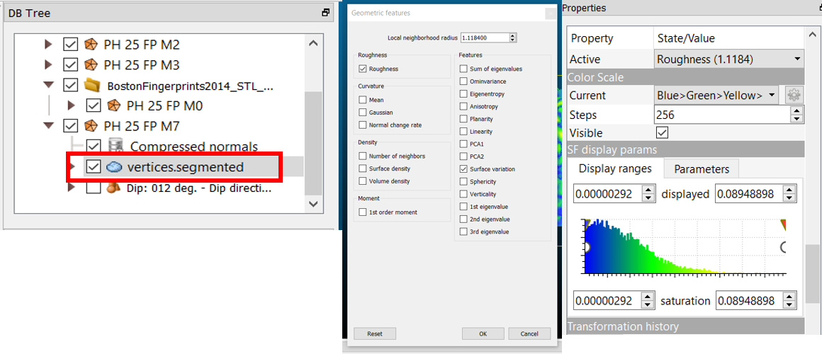
   a. To calculate roughness and surface variation for these fingerprints, ensure the ‘vertices’ component of the mesh is enabled and highlighted in the DB Tree.

   b. Then, navigate to the ‘Tools’ dropdown menu, and select ‘Other’. Choose ‘Compute Geometric Features’. A pop up window (shown in the image in the centre, below) will ask you which geometric features to calculate. Check both Roughness and Surface Variation. In the ‘Local neighbourhood radius’ box, the software will have provided a suggested kernel radius, but this will likely be too small to be useful. You can try playing with this setting to see the different results, but a relatively reliable number to input here is 1.1184.

   c. Whichever number you use here, you need to ensure that this number is the same for each of the fingerprints for this quantitative comparison to be valid. Click OK, and you will find both of these calculations saved as values under the mesh’s Scalar Field.

   d. In the mesh’s Properties, under ‘Color Scale’, ensure that ‘Roughness’ is selected initially and ensure you have checked the box next to the ‘Color Scale’ to ensure it is visible. Repeat this step for each of the fingerprints.

1. Begin alternating between 3D viewports to observe the differences in roughness between these fingerprints. Take note of the numbers at the extreme ends of the Color Scale on the right – which fingerprints have been calculated to have the roughest relative surface?

2. Now repeat the process using the ‘Surface Variation’ parameter as the Scalar Field – does this have different results from your ranking of fingerprints by roughness?

3. If we look at Roughness only, it is clear that PH 25’s fingerprint M7 is less rough than the others – the color scale for Roughness only reaches 0.089489. The upper limits of the color scale for the other fingerprints fall within a range of 0.179 – 0.239. If we look at Roughness, this could be an indicator that the fingerprint M7 was made on a separate occasion after the pot had dried, but before it was fired.

4. This difference is less apparent if we look at ‘Surface Variation’, but it is clear that fingerprints M1 and M3 are characterised by more surface variation of the other three. If we visually inspect these two prints in particular, there are distinct peaks that are [not]{.ul} characteristic of fingerprint ridges. This patterning is suggestive that the clay was wet when the fingerprint was made, so much so that the clay pulled away when the finger was removed from the surface of the pot, and some pooling occurred.

   a. To lend more credence to this analysis and its subsequent interpretation, some experimental archaeology might be necessary (away from the computer). If you have paint available, use it to make a fingerprint on a piece of paper. Now try using a bit too much paint – it may end up looking something like PH 25’s fingerprint M1 or M3.

Reflect, Write and Interpret!

• Under ‘3D views’, choose ‘Tile’ view and take a screenshot of your collection of fingerprint meshes with what you think is the most informative morphometric parameter applied as a Scalar field. Add this to your gallery. For the caption, discuss why you found this parameter most informative, and how it informs your interpretation of PH 25’s biography. Do you think all of the fingerprints were applied at once? Do you think they were made by different people? The same person at different times? Use quantitative evidence to support your interpretation.
• At what step of the pottery manufacturing process might the potter have picked up a damp pot? Could it be the pot was moved twice – once to take it from the pottery wheel to a shelf to dry, and again to move the mostly-dry pot (but malleable enough to leave fingerprint M7?) to the kiln?

A step-by-step video guide to Exercise 4 can be found here.

Back to Exercise 3

To Exercise 5: Simple Measurements in CloudCompare