Exercise 3: The Basics of CloudCompare

(Allow at least 1 hour for Exercise 3)

A step-by-step video guide to Exercise 3 can be found here.

Meshlab allowed us to quickly visualise the datasets and take simple measurements from the 3D models to familiarise ourselves with the dataset. To take our analysis to the next step, we will use a different software tool which is more intuitive and has better functionality for isolating individual features, CloudCompare. In this exercise you will learn to:

• Isolate individual mesh components for closer analysis;

• Organise data by renaming meshes and save our CloudCompare project;

• Align 3D data to enable more accurate morphometric calculations;

• Implement the visualisation options in CloudCompare, in this case by using simple ‘morphometric parameters’ from the mesh surface as Scalar Fields.

Using Cloud Compare

CloudCompare is another free software package that is useful in working with and analysing 3D datasets. Only a few basic functions will be discussed here, but CloudCompare's User’s Manual is virtually comprehensive in describing its many uses. In some ways, it is more intuitive than MeshLab, although creating a visualisation as informative as the ‘Radiance Scaling’ shader from MeshLab in CloudCompare requires more work.

One big difference between CloudCompare and MeshLab is that, while you can work with 3D meshes in CloudCompare, the software was initially designed to work with point clouds, as the name ‘CloudCompare’ suggests. As described above in the introduction of this document, the point cloud is the cluster of individual points that are recorded by a 3D recording technique, whether this was by photogrammetry, structured light scanning, or laser scanning. Some of CloudCompare’s functions will use the vertices of the mesh as ‘point clouds’. This will be particularly important in Exercises 4 and 5.

What is a ‘morphometric parameter’? What do they tell us?

Morphometric parameters are quantitative measurements that can be used to describe an object’s form. This includes measurements you will already be familiar with (length, width, volume), but can also include parameters like ‘Roughness’ or ‘Curvature’. By incorporating these parameters, features that would otherwise be difficult to see on the physical object become much more obvious when applied to the 3D model. In Exercise 3, we will begin with using the Z coordinates, which represent the relative height of the mesh surface.

Shaders vs Morphometrics While they can both be used to visualise data, Shaders function differently from Morphometric Parameters. As noted above in Exercise 1, Shaders take multiple factors into their calculation, including: lighting position and transparency, view position, material properties, and the shape of the 3D surface. Morphometrics are simpler in that they only take into account the shape of the 3D surface; however, there are a wide variety of morphometric parameters that can be used in morphometrics (height, length, width, roughness, curvature) and can be used in quantitative applications, which will be explored more fully in Exercises 4 and 5.

Roughness and Curvature ‘Roughness’ and ‘Curvature’ are calculated using statistics. As defined by CloudCompare…

• Roughness: “For each point, the ‘roughness’ value is equal to the distance between this point and the best fitting plane computed on its nearest neighbours.”
• Curvature: “The curvature at each point is estimated by best fitting a quadric around it based on its nearest neighbours.”

Both of these calculations rely on a ‘nearest neighbours’ approach. While this concept can be applied differently in different fields, essentially the software determines whether a point is ‘different’ by looking at its neighbours within a given radius defined by the user. If a point’s elevation is quite similar compared to the plane formed by its neighbouring points, it will not be attributed to a high ‘roughness’ value.

Getting Started

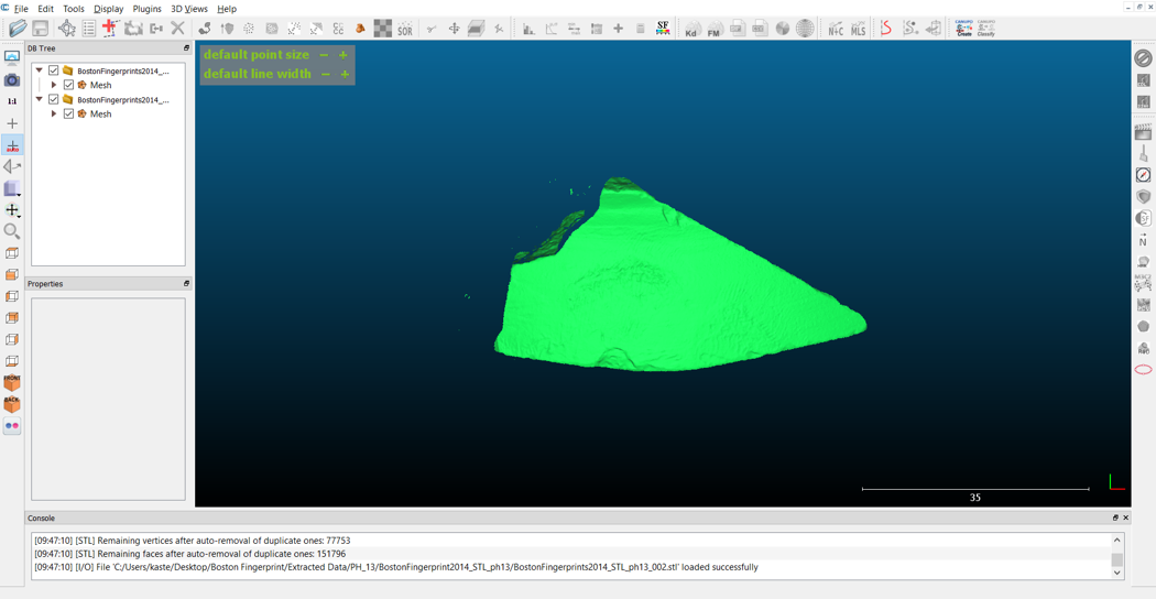
1. To start, ‘Open’ both of the .stl files from PH 13 (you can also use Ctrl+O). Your screen should look something like the image below.

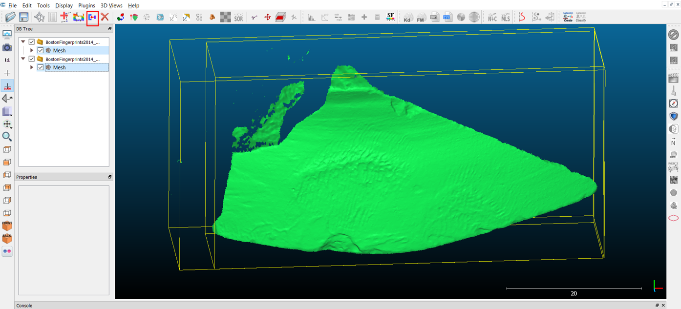
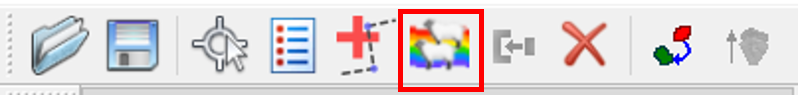
1. In the top left section of the workspace, you can see a window that says ‘DB Tree’ at the top (which is short for ‘DataBase Tree’). This is where you can see the files you have added to the project. Currently, the two .stl files we have imported are two separate entities. To merge the two files into one 3D entity, Ctrl+Click both of the ‘Mesh’ layers from each of the files so that these are both highlighted. Then, find and click the ‘Merge multiple clouds’ icon on the toolbar (highlighted with a red box below). Then, uncheck the boxes to the left of the original files so that only the new ‘Merged Mesh’ is visible.

1. Rotating the mesh is slightly different in CloudCompare, as the trackball is not constantly visible. Click and hold the mesh – the trackball will appear. Try moving your mouse to rotate the mesh. As you are moving the mesh, take note of the appearance of the fingerprint(s?). Let’s try isolating the fingerprints using the ‘Segment’ tool in CloudCompare.

Try it yourself!

• Kimberlee S Moran, a forensic archaeologist who specialises in ancient fingerprints, has produced a Fingerprinting Handout that introduces the key features fingerprint analysts use to differentiate between fingerprints. In this handout, we can see that the print in the centre of the sherd PH 13 does not exhibit any of the three basic print patterns: arch, loop, or whorl. Instead, these ridges all seem to be travelling parallel to each other (although the significantly raised clay in the centre makes it difficult to be certain). Examine your own fingers and hands – are there any areas that exhibit a similar pattern? What might have caused the raised area in the centre?
• As archaeologists, it is also important to consider at what stage of the manufacturing process these prints might have been made – the prints are made over the striations from the manufacturing processes, the clay was wet enough that prints were able to be made, and the prints were not effaced by the potter. What step in the manufacturing process might these prints represent? It could be that the print centrally positioned on the sherd represents a lower joint of the finger, rather than a fingertip. It could also be that this represents a partial hand-print, and that the clay ridge could have been caused by a palmar crease. If the former is true, the less well-defined print could be the fingerprint that we would want to examine, but is this detailed enough to identify features?

Segmenting in CloudCompare

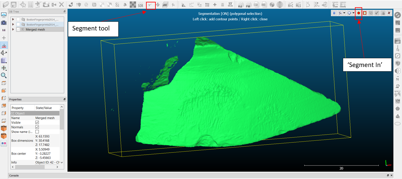
1. To do anything to alter the mesh, the ‘Merged Mesh’ will need to be highlighted in the DB Tree. The ‘Segment’ tool appears as a pair of scissors in the toolbar above the viewing window. Once you have selected the ‘Segment tool’, your screen should look something like that pictured below. As it says above the 3D model, left click around the fingerprints to add points to the polygon, and right click when you are happy with the shape you have created. Then, click the ‘Segment in’ to delete everything around the area you have selected.

1. Once you have selected ‘Segment In’, the Segmentation function will pause. You can now rotate the area you have selected to ensure you are happy with the results. If the area needs further editing, unpause the tool to continue segmenting. If you are satisfied with the results, click the checkmark in the Segment Toolbar to ‘Confirm Segmentation’.

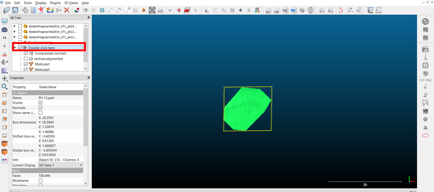
2. After confirming the segmentation, notice that the ‘Merged Mesh’ in the DB Tree has divided into two meshes: ‘Merged Mesh.remaining’ and ‘Merged Mesh.part’. Toggle each of these by clicking in the checkbox for each. You will see that your selected area has now been segmented from the rest of the 3D data. Turn off the ‘Merged Mesh.remaining’ layer to continue working with your fingerprint data.

Note: For better visualisation results, ensure that you have segmented each of the prints from each other so that you are only working with one print at a time. To rename the meshes in the DB Tree, double left click on the object name you wish to change (highlighted in red below).

Visualising 3D models in CloudCompare

Before making substantial edits, it is always a good idea to duplicate/clone the dataset you will be working with so that, if something goes wrong, you will not have to repeat the above steps each time. Highlight the Merged mesh.part and click the ‘Clone’ button (the icon shows two sheep, outlined in a red box below). If you want to save the work you have done in CloudCompare, you need to be sure that [all components] you want to save are highlighted in the DB Tree before you select ‘Save’ (you select multiple files/folders by holding down the ‘Ctrl’ button and clicking on the files you wish to save in the DB Tree).

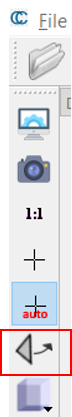
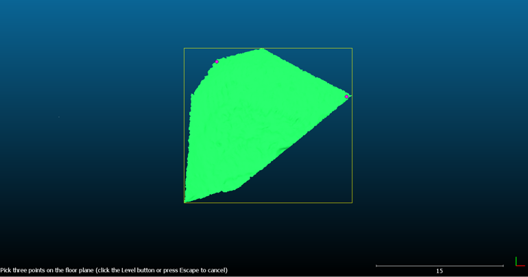
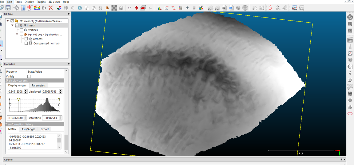
1. First, it is important that the fingerprint is as ‘flat’ as it can be in the 3D space, so that the software can recognise the high points and low points of the ridges (aligning the height of the ridges to represent the Z coordinates). From the toolbar on the left side of the screen, select the icon that looks like a black triangle and an arrow. The software will then prompt you to select three points on the 3D mesh. Ensure that these points are as far apart as possible on the mesh, along the edge, as this will determine how flat the print is.

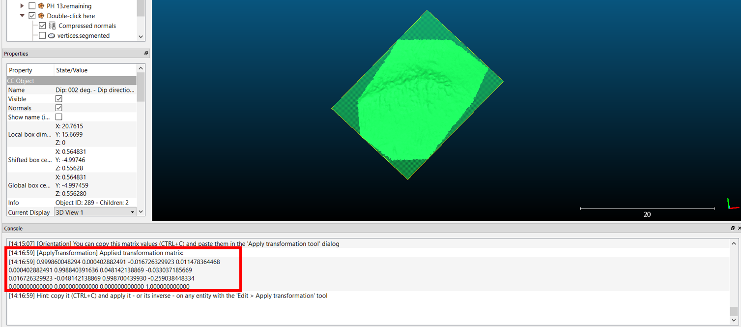
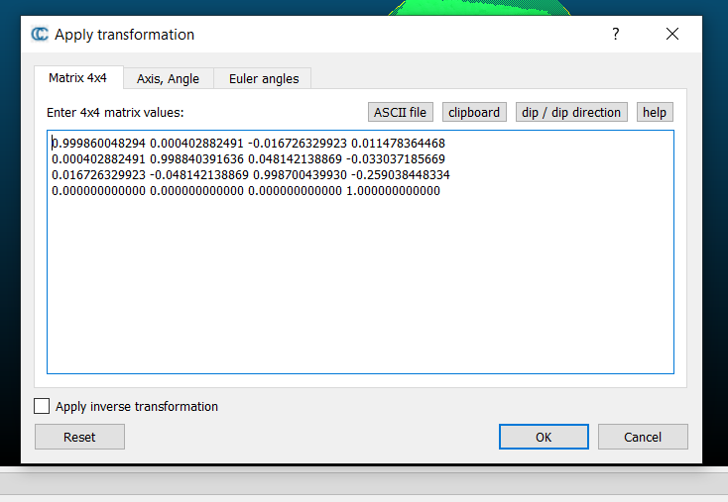
1. An automated option for levelling the mesh is provided under ‘Tools’, called ‘Fit’ to plane. This produces a transformation matrix in the ‘Console’ area of the screen (usually at the bottom of the window) that will align your mesh to the plane it has calculated. A matrix is an array that, in this case, dictates how the mesh needs to be mathematically rotated and translated to align with the plane. The first three columns correspond to how the points should rotate in three dimensions, while the fourth column corresponds to how much and in what direction the mesh needs to slide, or translate.

2. To apply this alignment, click on the matrix entry so that it is highlighted and use Ctrl+C to copy the matrix. Ensure that the mesh is highlighted in the DB tree. Navigate to the ‘Edit’ dropdown menu to find the ‘Apply Transformation’ function, delete the matrix provided and paste your new matrix in using Ctrl+V. Click ‘OK’ and the transformation will be complete. Uncheck the tick box next to the ‘Plane’ that was generated to remove it from view.

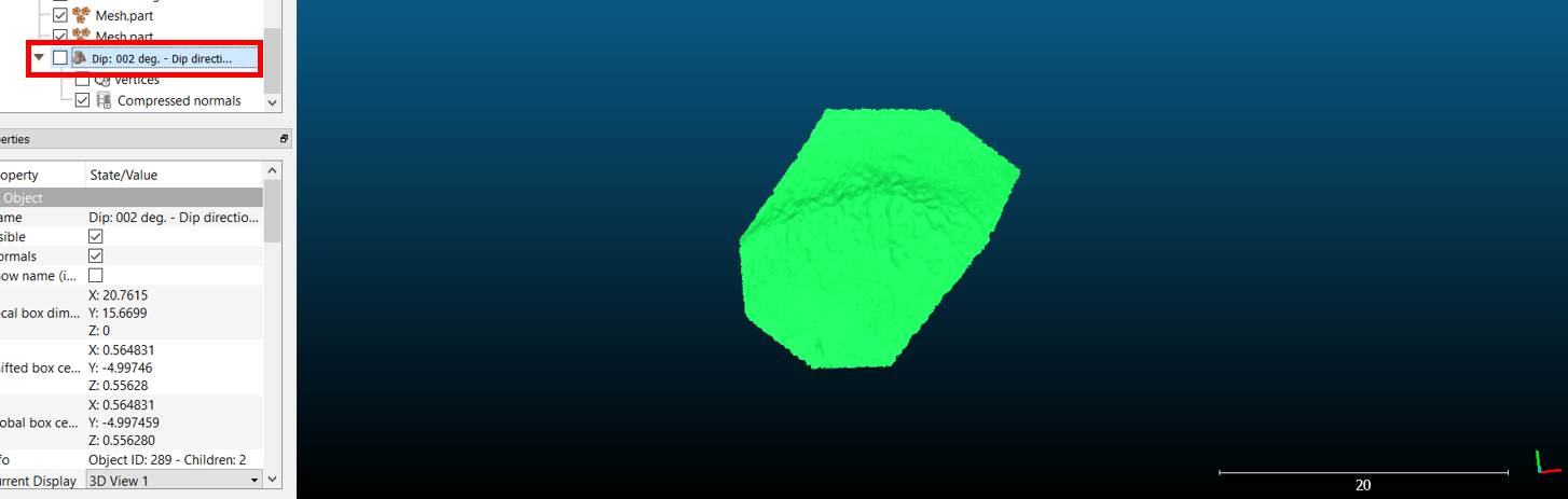
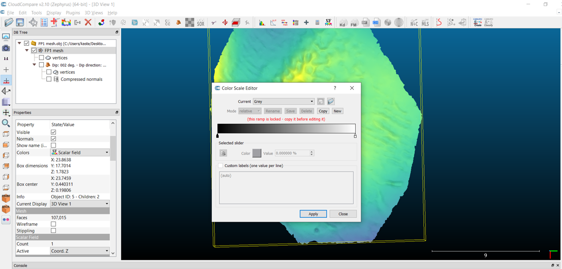
1. Once the 3D model is aligned, navigate to ‘Scalar Fields’ from the ‘Edit’ dropdown menu and select ‘Export coordinate(s) to SF(s)’. Ensure that the checkbox next to ‘Z’ is selected before you hit ‘Ok’. A Scalar Field, as defined in the CloudCompare manual, is ‘a set of values (one value per point)’; CloudCompare allows a value associated with a point/vertex to be displayed as colours or have filters or basic math operations applied to them. In this case, we are assigning the Z-values of the mesh as a scalar field – the relative height of the mesh above the level plane we created in the previous step(s). This will allow us to assign different colours to points with different heights. This is only one of many values that could be assigned to a Scalar Field; virtually any property that can be used to describe the shape of the surface can appear in the scalar field, including other morphometric parameters that will be introduced in Exercises 4 and 5.

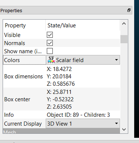
1. If you highlight the 3D model and navigate to the ‘Properties’ window (often automatically pinned below the DB Tree window), you will find that under ‘CC Object’ you can now change the ‘Colors’ from ‘None’ to ‘Scalar field’. Scrolling through the properties, under ‘Color Scale’, you will be able to change the appearance of the 3D model from a dropdown menu.

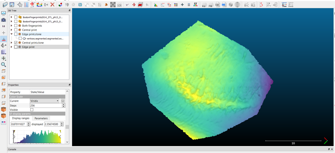
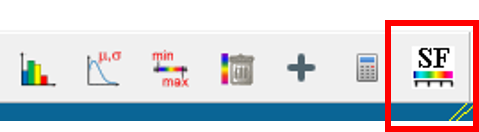
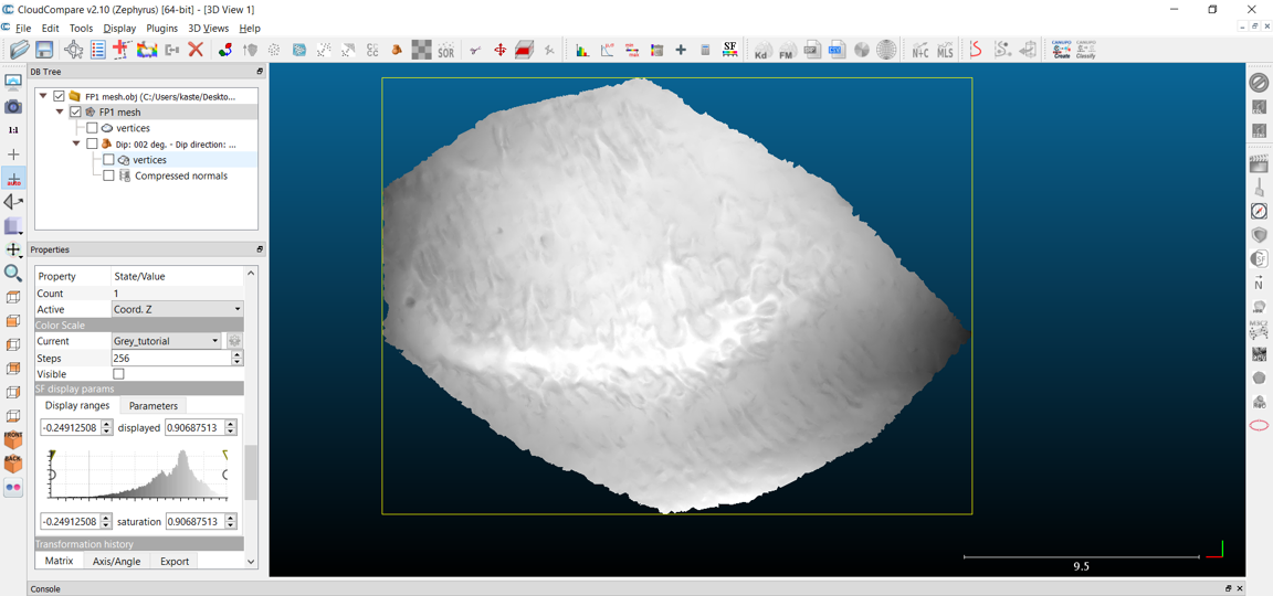
1. From the SF display params, using the Viridis setting (above), you can see that the highest values are yellow, while the lowest values are purple. This does not quite show the fingerprint at its best, though it clearly shows the ridge of raised clay in the centre of the print. To edit the colour scale, navigate to the icon for the ‘Color Scale Editor’ in the toolbar across the top of the screen. To edit any of the scales, you will first need to make a copy of the base color scale you start with. Choose to make a copy of the ‘Grey’ preset colours, rename the scale, and save it. Now set your new scale as the current color scale.

Reflect

• Notice that this preset Grey Color Scale does not reflect what one might expect from the image of a fingerprint – the raised ridges of the fingerprint receive the black ink and leave their impression on a piece of paper. The ‘peaks’ of the fingerprint then make up the darkest part of a fingerprint, while the ‘valleys’ create the white space in between. This preset Grey Color Scale instead assumes that the highest points of the 3D model should be bright and low points should be dark.
• Why is it that we expect the lower points on a 3D model to be dark and the brighter points on a 3D model to be bright? Are there any real-world situations that would lead to this expectation? Try picturing a mountainous landscape – as the sun moves across the sky, how does this affect the lighting of this landscape?
• If we were analysing a 3D model (something other than fingerprints), is it more useful to match the expectation conveyed by the preset Grey Color Scale? Why?

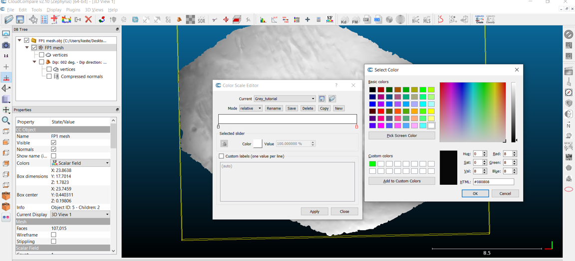
1. Now go back and edit your edited scalar field. On the color bar, you will see two small boxes at either end of the bar. Click on the black box on the left – you will see that the fields below this, in an area labelled ‘Selected Slider’, are now no longer greyed out. Change the colour of this end of the slider by clicking the box next to ‘Color’. For now, change this to white.

1. Now change the slider on the right side of the bar to black. Click apply and save the modifications.

2. Your screen should look something like the image below, with the black and white gradient inverted from its previous state. In the properties of the mesh, in the SF display params, experiment with sliding the triangles along the histogram to see how this affects the coloration of the 3D model.

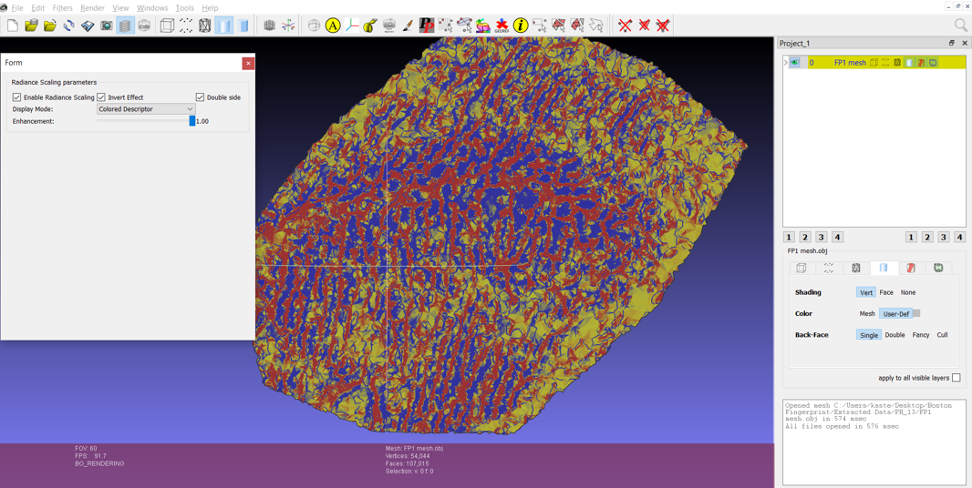
1. While the above image appears more similar to how we might visualise a fingerprint, the raised ridge of clay along the centre is clearly affecting how this is being visualised. If one were to compare this against some of the options in Meshlab’s Radiance Scaling (see below; the red areas highlight the raised ridges of the fingerprint), it is clear that the added topography from the ridge and the curvature of the ceramic vessel itself is diminishing the impact of the relative difference in height (the Z coordinates of the 3D model) between the fingerprint ridges and the dips between them.

Reflect and Write

• Try these visualisation processes with a flatter fingerprint from a different potsherd of your choice – do you run across the same issues? Does the curvature of the potsherd itself have a significant impact on the Z coordinates of the fingerprint?
• Take a screenshot of what you think is an informative visualisation of a fingerprint from any of the potsherds in the Boston Fingerprints archive, and add this to your gallery – what are the benefits to this visualisation over the others explored here? Write an extended caption explaining why.

Try it yourself!

• Are these 3D models from the Boston Fingerprints Project detailed enough that you can identify any of the six different ridge paths described by Kimberlee Moran in her handout (using visualisations from either CloudCompare or Meshlab)?
• Fingerprints are interesting to professionals in a variety of fields and we can use tools developed to investigate modern prints to look at our digital prints on ceramics. If fingerprints can be matched between potsherds from different contemporary sites, this will give us insight into trade routes or the movements of the individual potter.
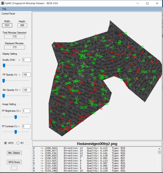
• Optional: If you want to try running one of the fingerprints you’ve identified through the Fingerprint Minutiae Viewer software (see image below), be sure to use the ‘Save Snapshot’ function in Meshlab so that the trackball is not visible in the image. You will also need an image editing software (like Adobe Photoshop) to convert your image to 8-bit greyscale.
  • Ensure that the raised areas of the fingerprint (in this case, the areas highlighted in red) are black in the image. In Adobe Photoshop, you can change the reds to black by using Image > Adjustments > Black & White and adjusting the ‘Reds’ slider so that the ridges appear black (but be sure that the strange ‘squiggly lines’ of noise are not overemphasised in this process).
  • Then use Image > Mode > Greyscale to convert it to Greyscale and ensure that the 8-bit option is checked. Then export the image as a .png file.
  • Once you have installed FMV, you can open your new image of the fingerprint in the software and see what Minutiae are identified. Be sure to critically analyse these – do the features highlighted in green appear to be reliable, distinctive features, as highlighted in Kimberlee Moran’s handout, or do they appear to be digital artefacts?

A step-by-step video guide to Exercise 3 can be found here.

Back to Exercise 2

To Exercise 4: Quantitative Approaches to Interpretation